

Python 机器学习秘籍(二)
五、构建推荐引擎
在本章中,我们将介绍以下食谱:
- 为数据处理构建函数组合
- 构建机器学习管道
- 寻找最近的邻居
- 构建 k 近邻分类器
- 构造 k 近邻回归器
- 计算欧几里德距离分数
- 计算皮尔逊相关分数
- 在数据集中查找相似的用户
- 生成电影推荐
简介
推荐引擎是一个可以预测用户可能感兴趣的模型。当我们把这个应用到电影的上下文中,这就变成了一个电影推荐引擎。我们通过预测当前用户对项目的评价来过滤数据库中的项目。这有助于我们将用户与数据集中正确的内容联系起来。为什么这是相关的?如果你有一个庞大的目录,那么用户可能会也可能不会找到所有相关的内容。通过推荐合适的内容,你增加了消费。网飞等公司非常依赖推荐来吸引用户。
推荐引擎通常使用协作过滤或基于内容的过滤来产生一组推荐。这两种方法的区别在于挖掘建议的方式。协同过滤根据当前用户过去的行为以及其他用户给出的评分来构建模型。然后我们使用这个模型来预测这个用户可能感兴趣的东西。另一方面,基于内容的过滤使用项目本身的特征,以便向用户推荐更多的项目。项目之间的相似性是这里的主要驱动力。在这一章中,我们将重点讨论协同过滤。
构建用于数据处理的函数组合
任何机器学习系统的主要部分之一是数据处理管道。在将数据输入机器学习算法进行训练之前,我们需要以不同的方式对其进行处理,以使其适合该算法。拥有一个强大的数据处理管道对于构建一个精确且可扩展的机器学习系统大有帮助。有许多基本功能可用,数据处理管道通常由这些功能的组合组成。与其以嵌套或循环的方式调用这些函数,不如使用函数式编程范式来构建组合。让我们来看看如何将这些函数组合起来,形成一个可重用的函数组合。在这个食谱中,我们将创建三个基本函数,并看看如何组成一个管道。
怎么做…
-
新建一个 Python 文件,添加如下一行:
import numpy as np -
让我们定义一个函数,将
3添加到数组的每个元素中:def add3(input_array): return map(lambda x: x+3, input_array) -
让我们定义第二个函数将
2与数组的每个元素相乘:def mul2(input_array): return map(lambda x: x*2, input_array) -
让我们定义第三个函数,从数组的每个元素中减去【T0:
def sub5(input_array): return map(lambda x: x-5, input_array) -
Let's define a function composer that takes functions as input arguments and returns a composed function. This composed function is basically a function that applies all the input functions in sequence:
def function_composer(*args):
    return reduce(lambda f, g: lambda x: f(g(x)), args)
我们使用
reduce函数,通过依次应用这些函数来组合所有的输入函数。 -
我们现在已经准备好使用这个函数编辑器了。让我们定义一些数据和一系列操作:
if __name__=='__main__': arr = np.array([2,5,4,7]) print "\nOperation: add3(mul2(sub5(arr)))" -
如果我们使用常规方法,我们将依次应用此方法,如下所示:
arr1 = add3(arr) arr2 = mul2(arr1) arr3 = sub5(arr2) print "Output using the lengthy way:", arr3 -
让我们用函数 composer 在一行中实现同样的事情:
func_composed = function_composer(sub5, mul2, add3) print "Output using function composition:", func_composed(arr) -
我们也可以用前面的方法在一行中做同样的事情,但是符号变得非常嵌套和不可读。还有,这是不能重复使用的!如果你想重用这个操作序列,你必须重新写一遍整件事:
print "\nOperation: sub5(add3(mul2(sub5(mul2(arr)))))\nOutput:", \ function_composer(mul2, sub5, mul2, add3, sub5)(arr) -
If you run this code, you will get the following output on the Terminal:

构建机器学习管道
scikit-learn 库提供了构建机器学习管道的功能。我们只需要指定函数,它将构建一个复合对象,使数据通过整个管道。该管道可以包括预处理、特征选择、监督学习、无监督学习等功能。在本食谱中,我们将构建一个管道来获取输入特征向量,选择顶部的 k 特征,然后使用随机森林分类器对它们进行分类。
怎么做…
-
新建一个 Python 文件,导入以下包:
from sklearn.datasets import samples_generator from sklearn.ensemble import RandomForestClassifier from sklearn.feature_selection import SelectKBest, f_regression from sklearn.pipeline import Pipeline -
Let's generate some sample data to play with:
# generate sample data
X, y = samples_generator.make_classification(
        n_informative=4, n_features=20, n_redundant=0, random_state=5)
这条线生成
20维特征向量,因为这是默认值。您可以使用上一行中的n_features参数进行更改。 -
管道的第一步是选择 k 最佳特征,然后进一步使用数据点。在这种情况下,让我们将
k设置为10:# Feature selector selector_k_best = SelectKBest(f_regression, k=10) -
下一步是使用随机森林分类器对数据进行分类:
# Random forest classifier classifier = RandomForestClassifier(n_estimators=50, max_depth=4) -
We are now ready to build the pipeline. The pipeline method allows us to use predefined objects to build the pipeline:
# Build the machine learning pipeline
pipeline_classifier = Pipeline([('selector', selector_k_best), ('rf', classifier)])
我们还可以为管道中的块指定名称。在前一行中,我们将
selector名称分配给我们的特征选择器,rf分配给我们的随机森林分类器。你可以在这里随意使用任何其他名字! -
我们还可以在进行的同时更新这些参数。我们可以使用上一步中指定的名称来设置参数。例如,如果我们想在特征选择器中将
k设置为6,在随机森林分类器中将n_estimators设置为25,我们可以像下面的代码中那样做。请注意,这些是上一步中给出的变量名:pipeline_classifier.set_params(selector__k=6, rf__n_estimators=25) -
让我们继续训练分类器:
# Training the classifier pipeline_classifier.fit(X, y) -
让我们预测训练数据的输出:
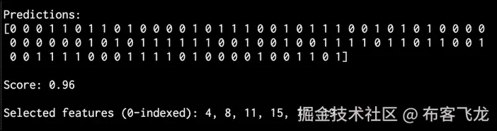
# Predict the output prediction = pipeline_classifier.predict(X) print "\nPredictions:\n", prediction -
让我们估计一下这个分类器的性能:
# Print score print "\nScore:", pipeline_classifier.score(X, y) -
我们还可以看到哪些功能被选中。让我们继续打印它们:
```py
# Print the selected features chosen by the selector
features_status = pipeline_classifier.named_steps['selector'].get_support()
selected_features = []
for count, item in enumerate(features_status):
    if item:
        selected_features.append(count)

print "\nSelected features (0-indexed):", ', '.join([str(x) for x in selected_features])
```
11. If you run this code, you will get the following output on your Terminal:
它是如何工作的…
选择 k 最佳特征的优势在于,我们将能够处理低维数据。这有助于降低计算复杂度。我们选择 k 最佳特征的方式是基于单变量特征选择。这将执行单变量统计测试,然后从特征向量中提取表现最好的特征。单变量统计检验是指涉及单个变量的分析技术。
一旦这些测试被执行,特征向量中的每个特征都被分配一个分数。基于这些分数,我们选择顶部的 k 特征。我们将此作为分类器管道中的预处理步骤。一旦我们提取了顶部的 k 特征,就形成了一个 k 维特征向量,并将其用作随机森林分类器的输入训练数据。
寻找最近的邻居
最近邻模型是指一类通用算法,旨在根据训练数据集中最近邻的数量做出决策。让我们看看如何找到最近的邻居。
怎么做…
-
新建一个 Python 文件,导入以下包:
import numpy as np import matplotlib.pyplot as plt from sklearn.neighbors import NearestNeighbors -
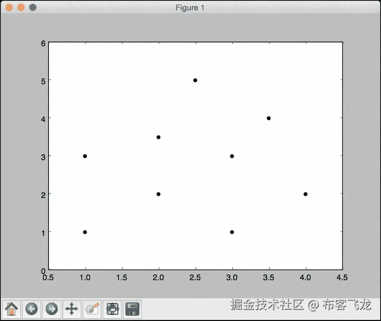
让我们创建一些示例二维数据:
# Input data X = np.array([[1, 1], [1, 3], [2, 2], [2.5, 5], [3, 1], [4, 2], [2, 3.5], [3, 3], [3.5, 4]]) -
我们的目标是找到任意给定点的三个最近邻居。我们来定义这个参数:
# Number of neighbors we want to find num_neighbors = 3 -
让我们定义一个不在输入数据中的随机数据点:
# Input point input_point = [2.6, 1.7] -
我们需要看看这些数据是什么样的。我们来绘制一下,如下:
# Plot datapoints plt.figure() plt.scatter(X[:,0], X[:,1], marker='o', s=25, color='k') -
为了找到最近的邻居,我们需要用正确的参数定义
NearestNeighbors对象,并在输入数据上训练它:# Build nearest neighbors model knn = NearestNeighbors(n_neighbors=num_neighbors, algorithm='ball_tree').fit(X) -
我们现在可以找到输入点到输入数据中所有点的距离:
distances, indices = knn.kneighbors(input_point) -
We can print the k-nearest neighbors, as follows:
# Print the 'k' nearest neighbors print "\nk nearest neighbors" for rank, index in enumerate(indices[0][:num_neighbors]): print str(rank+1) + " -->", X[index]indices数组已经排序,所以我们只需要解析它并打印数据点。 -
让我们绘制输入数据点并突出显示
k-最近的邻居:# Plot the nearest neighbors plt.figure() plt.scatter(X[:,0], X[:,1], marker='o', s=25, color='k') plt.scatter(X[indices][0][:][:,0], X[indices][0][:][:,1], marker='o', s=150, color='k', facecolors='none') plt.scatter(input_point[0], input_point[1], marker='x', s=150, color='k', facecolors='none') plt.show() -
If you run this code, you will get the following output on your Terminal:

- Here is the plot of the input datapoints:
- The second output figure depicts the location of the test datapoint and the three nearest neighbors, as shown in the following screenshot:

构建 k 近邻分类器
k 最近邻是算法,利用训练数据集中的 k 最近邻来寻找未知物体的类别。当我们想要找到一个未知点所属的类时,我们会找到 k 近邻,并进行多数投票。让我们来看看如何构造这个。
怎么做…
-
新建一个 Python 文件,导入以下包:
import numpy as np import matplotlib.pyplot as plt import matplotlib.cm as cm from sklearn import neighbors, datasets from utilities import load_data -
We will use the
data_nn_classifier.txtfile for input data. Let's load this input data:# Load input data input_file = 'data_nn_classifier.txt' data = load_data(input_file) X, y = data[:,:-1], data[:,-1].astype(np.int)前两列包含输入数据,最后一列包含标签。因此,我们将它们分为
X和y,如前面的代码所示。 -
Let's visualize the input data:
# Plot input data
plt.figure()
plt.title('Input datapoints')
markers = '^sov<>hp'
mapper = np.array([markers[i] for i in y])
for i in range(X.shape[0]):
    plt.scatter(X[i, 0], X[i, 1], marker=mapper[i],
            s=50, edgecolors='black', facecolors='none')
我们遍历所有的数据点,并使用适当的标记来分隔类。
-
为了构建分类器,我们需要指定我们想要考虑的最近邻居的数量。我们来定义这个参数:
# Number of nearest neighbors to consider num_neighbors = 10 -
为了可视化边界,我们需要定义一个网格,并评估该网格上的分类器。让我们定义步长:
# step size of the grid h = 0.01 -
我们现在准备构建 k 近邻分类器。让我们定义并训练它:
# Create a K-Neighbours Classifier model and train it classifier = neighbors.KNeighborsClassifier(num_neighbors, weights='distance') classifier.fit(X, y) -
我们需要创建一个网格来绘制边界。让我们对此进行定义,如下所示:
# Create the mesh to plot the boundaries x_min, x_max = X[:, 0].min() - 1, X[:, 0].max() + 1 y_min, y_max = X[:, 1].min() - 1, X[:, 1].max() + 1 x_grid, y_grid = np.meshgrid(np.arange(x_min, x_max, h), np.arange(y_min, y_max, h)) -
让我们评估所有点的分类器输出:
# Compute the outputs for all the points on the mesh predicted_values = classifier.predict(np.c_[x_grid.ravel(), y_grid.ravel()]) -
让我们绘制一下,如下:
# Put the computed results on the map predicted_values = predicted_values.reshape(x_grid.shape) plt.figure() plt.pcolormesh(x_grid, y_grid, predicted_values, cmap=cm.Pastel1) -
现在我们绘制了颜色网格,让我们覆盖训练数据点,看看它们相对于边界的位置:
```py
# Overlay the training points on the map
for i in range(X.shape[0]):
    plt.scatter(X[i, 0], X[i, 1], marker=mapper[i],
            s=50, edgecolors='black', facecolors='none')

plt.xlim(x_grid.min(), x_grid.max())
plt.ylim(y_grid.min(), y_grid.max())
plt.title('k nearest neighbors classifier boundaries')
```
11. 现在,我们可以考虑一个测试数据点,看看分类器是否正确运行。让我们定义它并绘制出来:
```py
# Test input datapoint
test_datapoint = [4.5, 3.6]
plt.figure()
plt.title('Test datapoint')
for i in range(X.shape[0]):
    plt.scatter(X[i, 0], X[i, 1], marker=mapper[i],
            s=50, edgecolors='black', facecolors='none')

plt.scatter(test_datapoint[0], test_datapoint[1], marker='x',
        linewidth=3, s=200, facecolors='black')
```
12. 我们需要使用以下模型提取 k 近邻:
```py
# Extract k nearest neighbors
dist, indices = classifier.kneighbors(test_datapoint)
```
13. 让我们绘制 k 近邻并突出显示它们:
```py
# Plot k nearest neighbors
plt.figure()
plt.title('k nearest neighbors')

for i in indices:
    plt.scatter(X[i, 0], X[i, 1], marker='o',
            linewidth=3, s=100, facecolors='black')

plt.scatter(test_datapoint[0], test_datapoint[1], marker='x',
        linewidth=3, s=200, facecolors='black')

for i in range(X.shape[0]):
    plt.scatter(X[i, 0], X[i, 1], marker=mapper[i],
            s=50, edgecolors='black', facecolors='none')

plt.show()
```
14. 让我们在终端上打印分类器输出:
```py
print "Predicted output:", classifier.predict(test_datapoint)[0]
```
15. If you run this code, the first output figure depicts the distribution of the input datapoints:

16. The second output figure depicts the boundaries obtained using the k-nearest neighbors classifier:

17. The third output figure depicts the location of the test datapoint:

18. The fourth output figure depicts the location of the 10 nearest neighbors:

它是如何工作的…
k 近邻分类器存储所有可用的数据点,并基于相似性度量对新数据点进行分类。这种相似性度量通常以距离函数的形式出现。该算法是一种非参数技术,这意味着它在公式之前不需要找出任何底层参数。我们所需要做的就是选择一个对我们有用的k值。
一旦我们找到 k 最近的邻居,我们就获得多数票。一个新的数据点被 k 近邻的多数票分类。这个数据点被分配给 k 近邻中最常见的类。如果我们将k的值设置为1,那么这就变成了最近邻分类器的情况,我们只需将数据点分配给训练数据集中最近邻的类。你可以在上了解更多。html 。
构造 k 近邻回归器
我们学习了如何使用 k 近邻算法构建分类器。好的一点是,我们也可以用这个算法作为回归器。让我们看看如何用它作为回归器。
怎么做…
-
新建一个 Python 文件,导入以下包:
import numpy as np import matplotlib.pyplot as plt from sklearn import neighbors -
让我们生成一些高斯分布的样本数据:
# Generate sample data amplitude = 10 num_points = 100 X = amplitude * np.random.rand(num_points, 1) - 0.5 * amplitude -
我们需要在数据中加入一些噪声,以引入一些随机性。添加噪声的目的是看我们的算法是否能够通过它,并且仍然以健壮的方式运行:
# Compute target and add noise y = np.sinc(X).ravel() y += 0.2 * (0.5 - np.random.rand(y.size)) -
让我们将其可视化如下:
# Plot input data plt.figure() plt.scatter(X, y, s=40, c='k', facecolors='none') plt.title('Input data') -
We just generated some data and evaluated a continuous-valued function on all these points. Let's define a denser grid of points:
# Create the 1D grid with 10 times the density of the input data
x_values = np.linspace(-0.5*amplitude, 0.5*amplitude, 10*num_points)[:, np.newaxis]
我们定义了这个更密集的网格,因为我们想在所有这些点上评估我们的回归器,看看它与我们的函数有多接近。
-
让我们定义我们想要考虑的最近邻居的数量:
# Number of neighbors to consider n_neighbors = 8 -
让我们使用前面定义的参数初始化和训练 k 近邻回归器:
# Define and train the regressor knn_regressor = neighbors.KNeighborsRegressor(n_neighbors, weights='distance') y_values = knn_regressor.fit(X, y).predict(x_values) -
让我们看看回归器如何通过将输入和输出数据重叠在一起来执行:
plt.figure() plt.scatter(X, y, s=40, c='k', facecolors='none', label='input data') plt.plot(x_values, y_values, c='k', linestyle='--', label='predicted values') plt.xlim(X.min() - 1, X.max() + 1) plt.ylim(y.min() - 0.2, y.max() + 0.2) plt.axis('tight') plt.legend() plt.title('K Nearest Neighbors Regressor') plt.show() -
If you run this code, the first figure depicts the input datapoints:
-
The second figure depicts the predicted values by the regressor:

它是如何工作的…
回归器的目标是预测连续的有价值的产出。在这种情况下,我们没有固定数量的输出类别。我们只有一组实值输出值,我们希望我们的回归器预测未知数据点的输出值。在这种情况下,我们使用sinc函数来演示 k 近邻回归器。这也被称为基数正弦函数。一个sinc功能定义如下:
当 x 不为 0 时 sinc(x)= sin(x)/x
= x 为 0 时为 1
当x为0时, sin(x)/x 取 0/0 的不定形。因此,我们必须计算这个函数的极限,因为x趋向于0。我们使用一组值进行训练,并定义了一个更密集的网格进行测试。从上图中我们可以看到,输出曲线接近训练输出。
计算欧几里德距离得分
现在我们已经有了足够的机器学习管道和最近邻分类器的背景,让我们开始讨论推荐引擎。为了构建一个推荐引擎,我们需要定义一个相似性度量,这样我们就可以在数据库中找到与给定用户相似的用户。欧几里得距离分数就是这样一个度量,我们可以用它来计算数据点之间的距离。我们将集中讨论电影推荐引擎。让我们看看如何计算两个用户之间的欧几里得分数。
怎么做…
-
新建一个 Python 文件,导入以下包:
import json import numpy as np -
我们现在将定义一个函数来计算两个用户之间的欧几里得分数。第一步是检查数据库中是否有用户:
# Returns the Euclidean distance score between user1 and user2 def euclidean_score(dataset, user1, user2): if user1 not in dataset: raise TypeError('User ' + user1 + ' not present in the dataset') if user2 not in dataset: raise TypeError('User ' + user2 + ' not present in the dataset') -
为了计算分数,我们需要提取两个用户都评分的电影:
# Movies rated by both user1 and user2 rated_by_both = {} for item in dataset[user1]: if item in dataset[user2]: rated_by_both[item] = 1 -
如果没有共同的电影,那么用户之间就没有相似性(或者至少根据数据库中的评分我们无法计算出来):
# If there are no common movies, the score is 0 if len(rated_by_both) == 0: return 0 -
For each of the common ratings, we just compute the square root of the sum of squared differences and normalize it so that the score is between 0 and 1:
    squared_differences = []

    for item in dataset[user1]:
        if item in dataset[user2]:
            squared_differences.append(np.square(dataset[user1][item] - dataset[user2][item]))

    return 1 / (1 + np.sqrt(np.sum(squared_differences)))
如果评级相似,那么平方差之和将非常低。因此,分数会变得很高,这也是我们希望从这个指标中得到的。
-
我们将使用
movie_ratings.json文件作为我们的数据文件。让我们加载它:if __name__=='__main__': data_file = 'movie_ratings.json' with open(data_file, 'r') as f: data = json.loads(f.read()) -
让我们考虑两个随机用户,计算欧几里得距离分数:
user1 = 'John Carson' user2 = 'Michelle Peterson' print "\nEuclidean score:" print euclidean_score(data, user1, user2) -
当您运行此代码时,您将看到终端上打印的欧几里德距离分数。
计算皮尔逊相关得分
欧几里德距离分数是一个很好的度量,但是它有一些缺点。因此,皮尔逊相关得分经常被用在推荐引擎中。让我们看看如何计算它。
怎么做…
-
新建一个 Python 文件,导入以下包:
import json import numpy as np -
我们将定义一个函数来计算数据库中两个用户之间的皮尔逊相关分数。我们的第一步是确认这些用户存在于数据库中:
# Returns the Pearson correlation score between user1 and user2 def pearson_score(dataset, user1, user2): if user1 not in dataset: raise TypeError('User ' + user1 + ' not present in the dataset') if user2 not in dataset: raise TypeError('User ' + user2 + ' not present in the dataset') -
下一步是获得这两个用户都评价的电影:
# Movies rated by both user1 and user2 rated_by_both = {} for item in dataset[user1]: if item in dataset[user2]: rated_by_both[item] = 1 num_ratings = len(rated_by_both) -
如果没有共同的电影,那么这些用户之间就没有可辨别的相似性;因此,我们返回
0:# If there are no common movies, the score is 0 if num_ratings == 0: return 0 -
我们需要计算常见电影评分的平方值之和:
# Compute the sum of ratings of all the common preferences user1_sum = np.sum([dataset[user1][item] for item in rated_by_both]) user2_sum = np.sum([dataset[user2][item] for item in rated_by_both]) -
让我们计算所有常见电影评分的平方总和:
# Compute the sum of squared ratings of all the common preferences user1_squared_sum = np.sum([np.square(dataset[user1][item]) for item in rated_by_both]) user2_squared_sum = np.sum([np.square(dataset[user2][item]) for item in rated_by_both]) -
让我们计算乘积的总和:
# Compute the sum of products of the common ratings product_sum = np.sum([dataset[user1][item] * dataset[user2][item] for item in rated_by_both]) -
我们现在准备计算皮尔逊相关分数所需的各种元素:
# Compute the Pearson correlation Sxy = product_sum - (user1_sum * user2_sum / num_ratings) Sxx = user1_squared_sum - np.square(user1_sum) / num_ratings Syy = user2_squared_sum - np.square(user2_sum) / num_ratings -
我们需要注意分母变成
0:if Sxx * Syy == 0: return 0的情况
-
如果一切正常,我们返回皮尔逊相关得分,如下所示:
```py
return Sxy / np.sqrt(Sxx * Syy)
```
11. 让我们定义main函数,计算两个用户之间的皮尔逊相关得分:
```py
if __name__=='__main__':
    data_file = 'movie_ratings.json'

    with open(data_file, 'r') as f:
        data = json.loads(f.read())
user1 = 'John Carson'
user2 = 'Michelle Peterson'
print "\nPearson score:"
print pearson_score(data, user1, user2)
```
12. 如果您运行此代码,您将看到皮尔逊相关分数打印在终端上。
在数据集中寻找相似用户
构建推荐引擎最重要的任务之一是找到相似的用户。这将指导您创建将提供给这些用户的建议。让我们看看如何建立这个。
怎么做…
-
新建一个 Python 文件,导入以下包:
import json import numpy as np from pearson_score import pearson_score -
让我们定义一个函数来查找与输入用户相似的用户。它需要三个输入参数:数据库、输入用户和我们正在寻找的相似用户的数量。我们的第一步是检查用户是否在数据库中。如果该用户存在,我们需要计算该用户与数据库中所有其他用户之间的皮尔逊相关得分:
# Finds a specified number of users who are similar to the input user def find_similar_users(dataset, user, num_users): if user not in dataset: raise TypeError('User ' + user + ' not present in the dataset') # Compute Pearson scores for all the users scores = np.array([[x, pearson_score(dataset, user, x)] for x in dataset if user != x]) -
下一步是按降序排列这些分数:
# Sort the scores based on second column scores_sorted = np.argsort(scores[:, 1]) # Sort the scores in decreasing order (highest score first) scored_sorted_dec = scores_sorted[::-1] -
让我们提取 k 的最高分并返回:
# Extract top 'k' indices top_k = scored_sorted_dec[0:num_users] return scores[top_k] -
让我们定义
main函数并加载输入数据库:if __name__=='__main__': data_file = 'movie_ratings.json' with open(data_file, 'r') as f: data = json.loads(f.read()) -
我们想找三个类似的用户,比如
John Carson。我们使用以下步骤进行操作:user = 'John Carson' print "\nUsers similar to " + user + ":\n" similar_users = find_similar_users(data, user, 3) print "User\t\t\tSimilarity score\n" for item in similar_users: print item[0], '\t\t', round(float(item[1]), 2) -
If you run this code, you will see the following printed on your Terminal:
生成电影推荐
现在我们已经构建了推荐引擎的所有不同部分,我们已经准备好生成电影推荐了。我们将使用我们在前面的食谱中构建的所有功能来构建一个电影推荐引擎。让我们看看如何构建它。
怎么做…
-
新建一个 Python 文件,导入以下包:
import json import numpy as np from euclidean_score import euclidean_score from pearson_score import pearson_score from find_similar_users import find_similar_users -
我们将定义一个函数来为给定用户生成电影推荐。第一步是检查用户是否存在于数据集中:
# Generate recommendations for a given user def generate_recommendations(dataset, user): if user not in dataset: raise TypeError('User ' + user + ' not present in the dataset') -
让我们计算该用户与数据集中所有其他用户的皮尔逊得分:
total_scores = {} similarity_sums = {} for u in [x for x in dataset if x != user]: similarity_score = pearson_score(dataset, user, u) if similarity_score <= 0: continue -
我们需要找到这个用户没有评分的电影:
for item in [x for x in dataset[u] if x not in dataset[user] or dataset[user][x] == 0]: total_scores.update({item: dataset[u][item] * similarity_score}) similarity_sums.update({item: similarity_score}) -
如果用户已经观看了数据库中的每一部电影,那么我们不能向该用户推荐任何内容。我们来处理一下这个情况:
if len(total_scores) == 0: return ['No recommendations possible'] -
我们现在有这些分数的列表。让我们创建一个标准化的电影排名列表:
# Create the normalized list movie_ranks = np.array([[total/similarity_sums[item], item] for item, total in total_scores.items()]) -
我们需要根据分数降序排序:
# Sort in decreasing order based on the first column movie_ranks = movie_ranks[np.argsort(movie_ranks[:, 0])[::-1]] -
我们终于准备好提取电影推荐:
# Extract the recommended movies recommendations = [movie for _, movie in movie_ranks] return recommendations -
让我们定义
main函数并加载数据集:if __name__=='__main__': data_file = 'movie_ratings.json' with open(data_file, 'r') as f: data = json.loads(f.read()) -
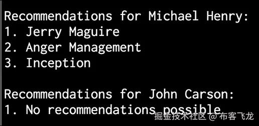
让我们为
Michael Henry:
```py
    user = 'Michael Henry'
    print "\nRecommendations for " + user + ":"
    movies = generate_recommendations(data, user)
    for i, movie in enumerate(movies):
        print str(i+1) + '. ' + movie
```

生成推荐
11. 用户John Carson已经看完了所有的电影。因此,如果我们试图为他生成推荐,它应该显示 0 个推荐。我们来看看是否会这样:
```py
    user = 'John Carson'
    print "\nRecommendations for " + user + ":"
    movies = generate_recommendations(data, user)
    for i, movie in enumerate(movies):
        print str(i+1) + '. ' + movie
```
12. If you run this code, you will see the following on your Terminal:
六、分析文本数据
在本章中,我们将介绍以下食谱:
- 使用标记化预处理数据
- 词干文本数据
- 使用引理化将文本转换为基本形式
- 使用分块分割文本
- 构建单词包模型
- 构建文本分类器
- 确定性别
- 分析句子的情感
- 使用主题建模识别文本中的模式
简介
文本分析和自然语言处理 ( NLP )是现代人工智能系统不可或缺的一部分。计算机擅长理解种类有限的严格结构化的数据。然而,当我们处理非结构化的自由格式文本时,事情开始变得困难。开发自然语言处理应用具有挑战性,因为计算机很难理解底层概念。我们交流事物的方式也有许多微妙的变化。这些可以是方言、上下文、俚语等形式。
为了解决这个问题,基于机器学习开发了自然语言处理应用。这些算法检测文本数据中的模式,以便我们可以从中提取见解。人工智能公司大量使用自然语言处理和文本分析来提供相关结果。自然语言处理最常见的应用包括搜索引擎、情感分析、主题建模、词性标注、实体识别等。自然语言处理的目标是开发一套算法,这样我们就可以用简单的英语与计算机交互。如果我们能做到这一点,那么我们就不需要编程语言来指导计算机应该做什么。在这一章中,我们将看看一些专注于文本分析的方法,以及我们如何从文本数据中提取有意义的信息。本章我们将大量使用名为自然语言工具包 ( NLTK )的 Python 包。确保安装后再继续。您可以在www.nltk.org/install.htm…找到安装步骤。您还需要安装 NLTK 数据,它包含许多语料库和训练好的模型。这是文本分析不可或缺的一部分!您可以在www.nltk.org/data.html找到安装步骤。
使用标记化预处理数据
标记化 是将文本分割成一组有意义的片段的过程。这些棋子被称为代币。举个的例子,我们可以把一大块文字分成单词,也可以把它分成句子。根据手头的任务,我们可以定义自己的条件,将输入文本分成有意义的标记。让我们看看如何做到这一点。
怎么做…
-
创建一个新的 Python 文件,并添加以下行。让我们定义一些示例文本进行分析:
text = "Are you curious about tokenization? Let's see how it works! We need to analyze a couple of sentences with punctuations to see it in action." -
让我们从句子标记化开始。NLTK 提供了一个句子标记器,所以让我们导入这个:
# Sentence tokenization from nltk.tokenize import sent_tokenize -
对输入文本运行句子标记器并提取标记:
sent_tokenize_list = sent_tokenize(text) -
打印句子列表,看看是否正确:
print "\nSentence tokenizer:" print sent_tokenize_list -
单词标记化在自然语言处理中非常常用。NLTK 附带了几个不同的单词标记器。让我们从基本单词标记器开始:
# Create a new word tokenizer from nltk.tokenize import word_tokenize print "\nWord tokenizer:" print word_tokenize(text) -
还有另一个单词标记器,叫做
PunktWord标记器。这会在标点符号上分割文本,但会将其保留在单词内:# Create a new punkt word tokenizer from nltk.tokenize import PunktWordTokenizer punkt_word_tokenizer = PunktWordTokenizer() print "\nPunkt word tokenizer:" print punkt_word_tokenizer.tokenize(text) -
如果你想把这些标点符号分成独立的符号,那么我们需要使用
WordPunct符号化器:# Create a new WordPunct tokenizer from nltk.tokenize import WordPunctTokenizer word_punct_tokenizer = WordPunctTokenizer() print "\nWord punct tokenizer:" print word_punct_tokenizer.tokenize(text) -
The full code is in the
tokenizer.pyfile. If you run this code, you will see the following output on your Terminal:
提取文本数据
当我们处理一个文本文档时,我们会遇到不同形式的单词。想想“玩”这个词。这个词可以以各种形式出现,比如“玩”“玩”“玩家”“玩”等等。这些基本上都是意义相似的词族。在文本分析过程中,提取这些单词的基本形式是很有用的。这将有助于我们提取一些统计数据来分析整个文本。词干的目标是将这些不同的形式简化为一个共同的基本形式。这使用启发式过程来切断单词的末端以提取基本形式。让我们看看如何在 Python 中做到这一点。
怎么做…
-
新建一个 Python 文件,导入以下包:
from nltk.stem.porter import PorterStemmer from nltk.stem.lancaster import LancasterStemmer from nltk.stem.snowball import SnowballStemmer -
我们来定义几个可以玩的词,如下:
words = ['table', 'probably', 'wolves', 'playing', 'is', 'dog', 'the', 'beaches', 'grounded', 'dreamt', 'envision'] -
我们将定义一个我们想要使用的词干分析器列表:
# Compare different stemmers stemmers = ['PORTER', 'LANCASTER', 'SNOWBALL'] -
初始化所有三个词干分析器所需的对象:
stemmer_porter = PorterStemmer() stemmer_lancaster = LancasterStemmer() stemmer_snowball = SnowballStemmer('english') -
为了以整洁的表格形式打印输出数据,我们需要以正确的方式格式化它:
formatted_row = '{:>16}' * (len(stemmers) + 1) print '\n', formatted_row.format('WORD', *stemmers), '\n' -
让我们遍历单词列表,并使用三个词干分析器对它们进行词干分析:
for word in words: stemmed_words = [stemmer_porter.stem(word), stemmer_lancaster.stem(word), stemmer_snowball.stem(word)] print formatted_row.format(word, *stemmed_words) -
The full code is in the
stemmer.pyfile. If you run this code, you will see the following output on your Terminal. Observe how the Lancaster stemmer behaves differently for a couple of words:
它是如何工作的…
所有三种词干算法基本上都是为了达到同样的目的。三种词干算法之间的区别基本上是它们操作的严格程度。如果您观察输出,您会看到兰开斯特词干分析器比其他两个词干分析器更严格。就严格程度而言,搬运工是最少的,兰开斯特是最严格的。我们从兰开斯特词干师那里得到的词干往往会变得混乱和模糊。算法确实很快,但是会减少很多单词。因此,一个很好的经验法则是使用雪球茎杆。
使用引理化将文本转换为基本形式
引理化的目标也是将单词简化为它们的基本形式,但这是一种更结构化的方法。在前面的食谱中,我们看到我们使用词干分析器获得的基本单词并没有真正的意义。例如,“狼”这个词被简化为“wolv”,这不是一个真实的词。引理化通过使用词汇和单词的形态学分析来解决这个问题。它删除屈折词尾,如“ing”或“ed”,并返回单词的基本形式。这种基本形式被称为引理。如果你把“狼”这个词具体化,你会得到“狼”作为输出。输出取决于标记是动词还是名词。让我们看看如何在这个食谱中做到这一点。
怎么做…
-
创建一个新的 Python 文件,导入如下包:
from nltk.stem import WordNetLemmatizer -
让我们定义我们在词干制作过程中使用的同一组词:
words = ['table', 'probably', 'wolves', 'playing', 'is', 'dog', 'the', 'beaches', 'grounded', 'dreamt', 'envision'] -
我们将比较两个引理器,
NOUN和VERB引理器。让我们把它们列举如下:# Compare different lemmatizers lemmatizers = ['NOUN LEMMATIZER', 'VERB LEMMATIZER'] -
基于
WordNet引理创建对象:lemmatizer_wordnet = WordNetLemmatizer() -
为了以表格形式打印输出,我们需要以正确的方式格式化输出:
formatted_row = '{:>24}' * (len(lemmatizers) + 1) print '\n', formatted_row.format('WORD', *lemmatizers), '\n' -
遍历单词并将其引理:
for word in words: lemmatized_words = [lemmatizer_wordnet.lemmatize(word, pos='n'), lemmatizer_wordnet.lemmatize(word, pos='v')] print formatted_row.format(word, *lemmatized_words) -
The full code is in the
lemmatizer.pyfile. If you run this code, you will see the following output. Observe howNOUNandVERBlemmatizers differ when they lemmatize the word "is" in the following image:
使用分块分割文本
分块 是指将输入的文本分割成基于任意随机条件的片段。这不同于标记化,因为不存在任何约束,并且块根本不需要有意义。这在文本分析过程中经常使用。当您处理非常大的文本文档时,您需要将其分成几个块进行进一步分析。在这个食谱中,我们将输入的文本分成若干部分,其中每一部分都有固定数量的单词。
怎么做…
-
新建一个 Python 文件,导入以下包:
import numpy as np from nltk.corpus import brown -
让我们定义一个函数来将文本分割成块。第一步是根据空格分割文本:
# Split a text into chunks def splitter(data, num_words): words = data.split(' ') output = [] -
初始化几个必需的变量:
cur_count = 0 cur_words = [] -
让我们遍历单词:
for word in words: cur_words.append(word) cur_count += 1 -
一旦你点击了所需的字数,重置变量:
if cur_count == num_words: output.append(' '.join(cur_words)) cur_words = [] cur_count = 0 -
将组块追加到输出变量,并返回:
output.append(' '.join(cur_words) ) return output -
我们现在可以定义
main函数。从布朗语料库中加载数据。我们将使用前一万个单词:if __name__=='__main__': # Read the data from the Brown corpus data = ' '.join(brown.words()[:10000]) -
定义每个组块的字数:
# Number of words in each chunk num_words = 1700 -
初始化几个相关变量:
chunks = [] counter = 0 -
对该文本数据调用
splitter功能,打印输出:
```py
    text_chunks = splitter(data, num_words)

    print "Number of text chunks =", len(text_chunks)
```
11. 完整代码在chunking.py文件中。如果您运行此代码,您将看到终端上打印出的块的数量。应该是 6!
构建单词包模型
当我们处理包含数百万个单词的文本文档时,我们需要将它们转换成某种数字表示。这样做的原因是为了使它们可用于机器学习算法。这些算法需要数字数据,以便分析它们并输出有意义的信息。这就是词汇袋的方法出现的地方。这基本上是一个模型从所有文档中的所有单词中学习一个词汇。之后,它通过构建文档中所有单词的直方图来为每个文档建模。
怎么做…
-
新建一个 Python 文件,导入以下包:
import numpy as np from nltk.corpus import brown from chunking import splitter -
我们来定义
main函数。从布朗语料库中加载输入数据:if __name__=='__main__': # Read the data from the Brown corpus data = ' '.join(brown.words()[:10000]) -
将文本数据分成五大块:
# Number of words in each chunk num_words = 2000 chunks = [] counter = 0 text_chunks = splitter(data, num_words) -
创建一个基于这些文本块的字典:
for text in text_chunks: chunk = {'index': counter, 'text': text} chunks.append(chunk) counter += 1 -
下一步是提取文档术语矩阵。这基本上是一个计算文档中每个单词出现次数的矩阵。我们将使用 scikit-learn 来做到这一点,因为与 NLTK 相比,它在这个特定的任务中有更好的规定。导入以下包:
# Extract document term matrix from sklearn.feature_extraction.text import CountVectorizer -
定义对象,提取文档术语矩阵:
vectorizer = CountVectorizer(min_df=5, max_df=.95) doc_term_matrix = vectorizer.fit_transform([chunk['text'] for chunk in chunks]) -
从
vectorizer对象中提取词汇并打印出来:vocab = np.array(vectorizer.get_feature_names()) print "\nVocabulary:" print vocab -
打印文档术语矩阵:
print "\nDocument term matrix:" chunk_names = ['Chunk-0', 'Chunk-1', 'Chunk-2', 'Chunk-3', 'Chunk-4'] -
要以表格形式打印,我们需要将其格式化,如下所示:
formatted_row = '{:>12}' * (len(chunk_names) + 1) print '\n', formatted_row.format('Word', *chunk_names), '\n' -
遍历单词,打印每个单词在不同组块中出现的次数:
```py
    for word, item in zip(vocab, doc_term_matrix.T):
        # 'item' is a 'csr_matrix' data structure
        output = [str(x) for x in item.data]
        print formatted_row.format(word, *output)
```
11. The full code is in the bag_of_words.py file. If you run this code, you will see two main things printed on the Terminal. The first output is the vocabulary as shown in the following image:

12. The second thing is the document term matrix, which is a pretty long. The first few lines will look like the following:

它是如何工作的…
考虑以下句子:
- 第一句:棕色的狗在跑。
- 第二句:黑狗在黑屋子里。
- 第三句:禁止在室内跑步。
如果你考虑这三句话,我们有以下九个独特的词:
- 这
- 棕色
- 狗
- 是
- 运转
- 黑色
- 在
- 房间
- 被禁止的
现在,让我们使用每个句子中的字数将每个句子转换成直方图。每个特征向量都是 9 维的,因为我们有 9 个唯一的词:
- 第一句:【1,1,1,1,0,0,0,0】
- 第二句:【2,0,1,1,0,2,1,1,0】
- 第三句:【0,0,0,1,1,0,1,1,1】
一旦我们提取出这些特征向量,就可以使用机器学习算法进行分析。
构建文本分类器
文本分类的目标是将文本文档分类为不同的类别。这是自然语言处理中极其重要的分析技术。我们将使用一种技术,该技术基于一个名为 tf-idf 的统计数据,该统计数据代表 术语频率—反向文档频率。这是一个分析工具,帮助我们理解一个单词对于一组文档中的一个文档有多重要。这是用来对文档进行分类的特征向量。你可以在www.tfidf.com了解更多。
怎么做…
-
新建一个 Python 文件,导入如下包:
from sklearn.datasets import fetch_20newsgroups -
让我们选择一个类别列表,并使用字典映射来命名它们。这些类别是我们刚刚导入的新闻组数据集的一部分:
category_map = {'misc.forsale': 'Sales', 'rec.motorcycles': 'Motorcycles', 'rec.sport.baseball': 'Baseball', 'sci.crypt': 'Cryptography', 'sci.space': 'Space'} -
根据我们刚刚定义的类别加载训练数据:
training_data = fetch_20newsgroups(subset='train', categories=category_map.keys(), shuffle=True, random_state=7) -
导入特征提取器:
# Feature extraction from sklearn.feature_extraction.text import CountVectorizer -
使用训练数据提取特征:
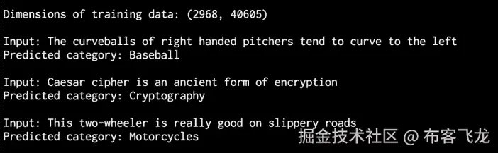
vectorizer = CountVectorizer() X_train_termcounts = vectorizer.fit_transform(training_data.data) print "\nDimensions of training data:", X_train_termcounts.shape -
我们现在已经准备好训练分类器了。我们将使用多项式朴素贝叶斯分类器:
# Training a classifier from sklearn.naive_bayes import MultinomialNB from sklearn.feature_extraction.text import TfidfTransformer -
定义几个随机输入的句子:
input_data = [ "The curveballs of right handed pitchers tend to curve to the left", "Caesar cipher is an ancient form of encryption", "This two-wheeler is really good on slippery roads" ] -
定义 tf-idf 转换器对象并对其进行训练:
# tf-idf transformer tfidf_transformer = TfidfTransformer() X_train_tfidf = tfidf_transformer.fit_transform(X_train_termcounts) -
一旦我们有了特征向量,使用这个数据训练多项式朴素贝叶斯分类器:
# Multinomial Naive Bayes classifier classifier = MultinomialNB().fit(X_train_tfidf, training_data.target) -
使用字数转换输入数据:
```py
X_input_termcounts = vectorizer.transform(input_data)
```
11. 使用 tf-idf 转换器转换输入数据:
```py
X_input_tfidf = tfidf_transformer.transform(X_input_termcounts)
```
12. 使用训练好的分类器预测这些输入句子的输出类别:
```py
# Predict the output categories
predicted_categories = classifier.predict(X_input_tfidf)
```
13. 打印输出,如下所示:
```py
# Print the outputs
for sentence, category in zip(input_data, predicted_categories):
    print '\nInput:', sentence, '\nPredicted category:', \
            category_map[training_data.target_names[category]]
```
14. The full code is in the tfidf.py file. If you run this code, you will see the following output printed on your Terminal:
它是如何工作的…
tf-idf 技术在信息检索中经常使用。目标是理解文档中每个单词的重要性。我们希望识别在文档中出现多次的单词。同时,像“是”和“是”这样的常用词并不能真正反映内容的本质。所以我们需要提取出真正的指标。每个单词的重要性随着字数的增加而增加。同时,随着它的大量出现,这个词的出现频率也增加了。这两件事往往会相互抵消。我们从每个句子中提取术语计数。一旦我们将其转换为特征向量,我们就训练分类器来对这些句子进行分类。
词频 ( TF ) 衡量一个单词在给定文档中出现的频率。由于多个文档的长度不同,直方图中的数字往往变化很大。因此,我们需要使之正常化,使之成为一个公平的竞争环境。为了实现规范化,我们将词频除以给定文档中的总字数。逆文档频率 ( IDF ) 衡量给定单词的重要性。当我们计算 TF 时,所有单词都被认为是同等重要的。为了平衡常用词的出现频率,我们需要把它们的权重降低,把稀有词的权重提高。我们需要计算带有给定单词的文档数量的比率,并将其除以文档总数。IDF 的计算方法是取这个比值的负算法。
例如,简单的单词,如“is”或“the”,往往会在各种文档中出现很多。然而,这并不意味着我们可以根据这些词来描述文档的特征。同时,如果一个单词出现一次,这也没有用。所以,我们寻找出现多次的单词,但不要太多,以免它们变得嘈杂。这是在 tf-idf 技术中制定的,用于对文档进行分类。搜索引擎经常使用这个工具来按相关性对搜索结果进行排序。
识别性别
在自然语言处理中,识别名字的性别是一项有趣的任务。我们将使用名称中最后几个字符是其定义特征的启发式方法。例如,如果名字以“la”结尾,则很可能是女性的名字,如“Angela”或“蕾拉”。另一方面,如果名字以“im”结尾,很可能是男性的名字,比如“Tim”或“Jim”。由于我们确定要使用的字符的确切数量,我们将对此进行实验。让我们看看怎么做。
怎么做…
-
新建一个 Python 文件,导入以下包:
import random from nltk.corpus import names from nltk import NaiveBayesClassifier from nltk.classify import accuracy as nltk_accuracy -
我们需要定义一个从输入单词中提取特征的函数:
# Extract features from the input word def gender_features(word, num_letters=2): return {'feature': word[-num_letters:].lower()} -
我们来定义
main函数。我们需要一些标注的训练数据:if __name__=='__main__': # Extract labeled names labeled_names = ([(name, 'male') for name in names.words('male.txt')] + [(name, 'female') for name in names.words('female.txt')]) -
播种随机数发生器,洗牌训练数据:
random.seed(7) random.shuffle(labeled_names) -
定义一些可以玩的输入名称:
input_names = ['Leonardo', 'Amy', 'Sam'] -
由于不知道需要考虑多少结尾字符,我们将参数空间从
1扫至5。每次,我们都会提取特征,如下所示:# Sweeping the parameter space for i in range(1, 5): print '\nNumber of letters:', i featuresets = [(gender_features(n, i), gender) for (n, gender) in labeled_names] -
将其分为训练和测试数据集:
train_set, test_set = featuresets[500:], featuresets[:500] -
我们将使用朴素贝叶斯分类器来做到这一点:
classifier = NaiveBayesClassifier.train(train_set) -
评估参数空间中每个值的分类器:
# Print classifier accuracy print 'Accuracy ==>', str(100 * nltk_accuracy(classifier, test_set)) + str('%') # Predict outputs for new inputs for name in input_names: print name, '==>', classifier.classify(gender_features(name, i)) -
The full code is in the
gender_identification.pyfile. If you run this code, you will see the following output printed on your Terminal:

分析句子的情绪
情感分析 是 NLP 最热门的应用之一。情感分析是指确定给定文本是积极的还是消极的过程。在一些变体中,我们认为“中性”是第三种选择。这种技术通常用于发现人们对某个特定话题的感受。这个用来分析用户各种形式的情绪,比如营销活动、社交媒体、电商客户等等。
怎么做…
-
新建一个 Python 文件,导入以下包:
import nltk.classify.util from nltk.classify import NaiveBayesClassifier from nltk.corpus import movie_reviews -
定义提取特征的函数:
def extract_features(word_list): return dict([(word, True) for word in word_list]) -
为此我们需要训练数据,所以我们将使用 NLTK 中的电影评论:
if __name__=='__main__': # Load positive and negative reviews positive_fileids = movie_reviews.fileids('pos') negative_fileids = movie_reviews.fileids('neg') -
让我们把这些分为正面和负面评论:
features_positive = [(extract_features(movie_reviews.words(fileids=[f])), 'Positive') for f in positive_fileids] features_negative = [(extract_features(movie_reviews.words(fileids=[f])), 'Negative') for f in negative_fileids] -
将数据分为训练和测试数据集:
# Split the data into train and test (80/20) threshold_factor = 0.8 threshold_positive = int(threshold_factor * len(features_positive)) threshold_negative = int(threshold_factor * len(features_negative)) -
提取特征:
features_train = features_positive[:threshold_positive] + features_negative[:threshold_negative] features_test = features_positive[threshold_positive:] + features_negative[threshold_negative:] print "\nNumber of training datapoints:", len(features_train) print "Number of test datapoints:", len(features_test) -
我们将使用朴素贝叶斯分类器。定义对象并训练:
# Train a Naive Bayes classifier classifier = NaiveBayesClassifier.train(features_train) print "\nAccuracy of the classifier:", nltk.classify.util.accuracy(classifier, features_test) -
分类器对象包含在分析过程中获得的信息量最大的单词。这些词基本上在被归类为积极或消极的评论中有很强的发言权。让我们打印出来:
print "\nTop 10 most informative words:" for item in classifier.most_informative_features()[:10]: print item[0] -
创建几个随机输入的句子:
# Sample input reviews input_reviews = [ "It is an amazing movie", "This is a dull movie. I would never recommend it to anyone.", "The cinematography is pretty great in this movie", "The direction was terrible and the story was all over the place" ] -
对这些输入句子运行分类器,获得预测:
```py
    print "\nPredictions:"
    for review in input_reviews:
        print "\nReview:", review
        probdist = classifier.prob_classify(extract_features(review.split()))
        pred_sentiment = probdist.max()
```
11. 打印输出:
```py
        print "Predicted sentiment:", pred_sentiment
        print "Probability:", round(probdist.prob(pred_sentiment), 2)
```
12. The full code is in the sentiment_analysis.py file. If you run this code, you will see three main things printed on the Terminal. The first is the accuracy, as shown in the following image:

13. The next is a list of most informative words:

14. The last is the list of predictions, which are based on the input sentences:

它是如何工作的…
我们在这里使用 NLTK 的朴素贝叶斯分类器来完成我们的任务。在特征提取器功能中,我们基本上提取所有唯一的单词。然而,NLTK 分类器需要数据以字典的形式排列。因此,我们以这样一种方式安排它,使得 NLTK 分类器对象可以摄取它。
一旦我们将数据划分为训练和测试数据集,我们就训练分类器将句子分为肯定和否定。如果你看一下顶部的信息词,你可以看到我们有“优秀”这样的词来表示正面评价,有“侮辱”这样的词来表示负面评价。这是一个有趣的信息,因为它告诉我们什么词被用来表示强烈的反应。
使用主题建模识别文本中的模式
主题建模 是指识别文本数据中隐藏的模式的过程。目标是在一组文档中发现一些隐藏的主题结构。这将帮助我们以更好的方式组织我们的文档,以便我们可以使用它们进行分析。这是自然语言处理中一个活跃的研究领域。你可以在www.cs.columbia.edu/~blei/topic…了解更多。在这个食谱中,我们将使用一个名为gensim的库。在继续之前,请确保安装了此软件。安装步骤见radimrehurek.com/gensim/inst…。
怎么做…
-
创建一个新的 Python 文件并导入以下包:
from nltk.tokenize import RegexpTokenizer from nltk.stem.snowball import SnowballStemmer from gensim import models, corpora from nltk.corpus import stopwords -
定义一个函数来加载输入数据。我们将使用已经提供给您的
data_topic_modeling.txt文本文件:# Load input data def load_data(input_file): data = [] with open(input_file, 'r') as f: for line in f.readlines(): data.append(line[:-1]) return data -
让我们定义一个类来预处理文本。这个预处理器负责创建所需的对象,并从输入文本中提取相关特征:
# Class to preprocess text class Preprocessor(object): # Initialize various operators def __init__(self): # Create a regular expression tokenizer self.tokenizer = RegexpTokenizer(r'\w+') -
我们需要一个停止单词的列表,这样我们就可以将它们排除在分析之外。这些都是常用词,如“在”、“该”、“是”等:
# get the list of stop words self.stop_words_english = stopwords.words('english') -
定义雪球茎干:
# Create a Snowball stemmer self.stemmer = SnowballStemmer('english') -
定义一个处理标记化、停止词移除和词干的处理器函数:
# Tokenizing, stop word removal, and stemming def process(self, input_text): # Tokenize the string tokens = self.tokenizer.tokenize(input_text.lower()) -
从文本中删除停止词:
# Remove the stop words tokens_stopwords = [x for x in tokens if not x in self.stop_words_english] -
对标记执行词干:
# Perform stemming on the tokens tokens_stemmed = [self.stemmer.stem(x) for x in tokens_stopwords] -
返回已处理的代币:
return tokens_stemmed -
我们现在准备定义
main函数。从文本文件加载输入数据:
```py
if __name__=='__main__':
    # File containing linewise input data
    input_file = 'data_topic_modeling.txt'

    # Load data
    data = load_data(input_file)
```
11. 定义一个基于我们定义的类的对象:
```py
    # Create a preprocessor object
    preprocessor = Preprocessor()
```
12. 我们需要处理文件中的文本,提取处理后的令牌:
```py
    # Create a list for processed documents
    processed_tokens = [preprocessor.process(x) for x in data]
```
13. 创建一个基于标记化文档的字典,以便可以用于主题建模:
```py
    # Create a dictionary based on the tokenized documents
    dict_tokens = corpora.Dictionary(processed_tokens)
```
14. 我们需要使用处理过的标记创建一个文档术语矩阵,如下所示:
```py
    # Create a document-term matrix
    corpus = [dict_tokens.doc2bow(text) for text in processed_tokens]
```
15. 假设我们知道文本可以分为两个主题。我们将使用一种称为 潜在狄利克雷分配 ( LDA )的技术进行主题建模。定义所需参数,初始化 LDA 模型对象:
```py
    # Generate the LDA model based on the corpus we just created
    num_topics = 2
    num_words = 4

    ldamodel = models.ldamodel.LdaModel(corpus,
            num_topics=num_topics, id2word=dict_tokens, passes=25)
```
16. 一旦确定了这两个主题,我们就可以通过查看贡献最大的单词来了解它是如何将这两个主题分开的:
```py
    print "Most contributing words to the topics:"
    for item in ldamodel.print_topics(num_topics=num_topics, num_words=num_words):
        print "\nTopic", item[0], "==>", item[1]
```
17. The full code is in the topic_modeling.py file. If you run this code, you will see the following printed on your Terminal:

它是如何工作的…
主题建模通过识别文档中主题的重要单词来工作。这些词往往决定了的话题是什么。我们使用正则表达式标记器,因为我们只需要没有任何标点符号或其他类型标记的单词。因此,我们使用它来提取标记。停止单词删除是另一个重要的步骤,因为这有助于我们消除由于单词引起的噪音,例如“is”或“the”。在这之后,我们需要把单词词干,以得到它们的基本形式。这整个东西被打包成文本分析工具中的预处理块。这也是我们在这里做的!
我们使用一种称为潜在狄利克雷分配(LDA)的技术来建模主题。LDA 基本上将文档表示为倾向于吐出单词的不同主题的混合。这些话是以一定的概率说出来的。目标是找到这些话题!这是一个生成模型,试图找到负责生成给定文档集的主题集。你可以在http://blog . echen . me/2011/08/22/潜在狄利克雷分配介绍了解更多。
从输出中可以看到,我们有“天赋”和“训练”这样的词来表征体育话题,而我们有“加密”来表征密码学话题。我们正在处理一个非常小的文本文件,这就是为什么有些单词看起来不太相关的原因。显然,如果使用更大的数据集,精度将会提高。
七、语音识别
在本章中,我们将介绍以下食谱:
- 读取和绘制音频数据
- 将音频信号转换到频域
- 生成带有自定义参数的音频信号
- 合成音乐
- 提取频域特征
- 建立隐马尔可夫模型
- 构建语音识别器
简介
语音识别是指识别和理解口语的过程。输入以音频数据的形式出现,语音识别器将处理这些数据,从中提取有意义的信息。这有很多实际用途,例如语音控制设备、将口语转录成单词、安全系统等等。
语音信号在本质上是多用途的。同一种语言有许多不同的说法。言语有不同的要素,如语言、情感、语气、噪音、口音等等。很难严格定义一套可以构成言语的规则。即使有所有这些变化,人类也非常善于相对容易地理解所有这些。因此,我们需要机器以同样的方式理解语音。
在过去的几十年里,研究人员致力于语音的各个方面,如识别说话者、理解单词、识别口音、翻译语音等。在所有这些任务中,自动语音识别一直是许多研究者关注的焦点。在本章中,我们将学习如何构建语音识别器。
读取和绘制音频数据
让我们来看看如何读取音频文件并可视化信号。这将是一个很好的起点,它将让我们对音频信号的基本结构有一个很好的了解。在开始之前,我们需要了解音频文件是实际音频信号的数字化版本。实际的音频信号是复杂的连续值波。为了保存数字版本,我们对信号进行采样并将其转换为数字。例如,语音通常以 44100 赫兹采样。这意味着信号的每一秒都被分解成 44100 个部分,并且存储这些时间戳的值。换句话说,每 1/44100 秒存储一个值。由于采样率高,当我们在媒体播放器上收听时,我们会感觉到信号是连续的。
怎么做…
-
新建一个 Python 文件,导入以下包:
import numpy as np import matplotlib.pyplot as plt from scipy.io import wavfile -
我们将使用
wavfile包从已经提供给您的input_read.wav输入文件中读取音频文件:# Read the input file sampling_freq, audio = wavfile.read('input_read.wav') -
让我们打印出这个信号的参数:
# Print the params print '\nShape:', audio.shape print 'Datatype:', audio.dtype print 'Duration:', round(audio.shape[0] / float(sampling_freq), 3), 'seconds' -
音频信号存储为 16 位有符号整数数据。我们需要标准化这些值:
# Normalize the values audio = audio / (2.**15) -
让我们提取前 30 个值进行绘图,如下所示:
# Extract first 30 values for plotting audio = audio[:30] -
X 轴是时间轴。让我们构建这个轴,考虑到它应该使用采样频率因子进行缩放的事实:
# Build the time axis x_values = np.arange(0, len(audio), 1) / float(sampling_freq) -
将单位转换为秒:
# Convert to seconds x_values *= 1000 -
让我们将绘制如下:
# Plotting the chopped audio signal plt.plot(x_values, audio, color='black') plt.xlabel('Time (ms)') plt.ylabel('Amplitude') plt.title('Audio signal') plt.show() -
The full code is in the
read_plot.pyfile. If you run this code, you will see the following signal: -
You will also see the following printed on your Terminal:

将音频信号转换到频域
音频信号由不同频率、振幅和相位的正弦波的复杂混合物组成。正弦波也被称为正弦波。音频信号的频率内容中隐藏着大量信息。事实上,音频信号的主要特征是其频率内容。整个的语言和音乐世界就是基于这个事实。在你继续之前,你需要一些关于傅立叶变换的知识。快速复习可以在www.thefouriertransform.com找到。现在,让我们看看如何将音频信号转换到频域。
怎么做…
-
新建一个 Python 文件,导入如下包:
import numpy as np from scipy.io import wavfile import matplotlib.pyplot as plt -
阅读已经提供给你的
input_freq.wav文件:# Read the input file sampling_freq, audio = wavfile.read('input_freq.wav') -
将信号标准化,如下所示:
# Normalize the values audio = audio / (2.**15) -
音频信号只是一个 NumPy 数组。因此,您可以使用以下代码提取长度:
# Extract length len_audio = len(audio) -
让我们应用傅立叶变换。傅立叶变换信号沿中心镜像,所以我们只需要取变换信号的前半部分。我们的最终目标是提取电力信号。因此,我们对信号中的值进行平方,为这个做准备:
# Apply Fourier transform transformed_signal = np.fft.fft(audio) half_length = np.ceil((len_audio + 1) / 2.0) transformed_signal = abs(transformed_signal[0:half_length]) transformed_signal /= float(len_audio) transformed_signal **= 2 -
提取信号的长度:
# Extract length of transformed signal len_ts = len(transformed_signal) -
我们需要根据信号的长度加倍信号:
# Take care of even/odd cases if len_audio % 2: transformed_signal[1:len_ts] *= 2 else: transformed_signal[1:len_ts-1] *= 2 -
使用以下公式提取功率信号:
# Extract power in dB power = 10 * np.log10(transformed_signal) -
X 轴是时间轴。我们需要根据采样频率进行缩放,然后将其转换为秒:
# Build the time axis x_values = np.arange(0, half_length, 1) * (sampling_freq / len_audio) / 1000.0 -
绘制信号,如下所示:
```py
# Plot the figure
plt.figure()
plt.plot(x_values, power, color='black')
plt.xlabel('Freq (in kHz)')
plt.ylabel('Power (in dB)')
plt.show()
```
11. The full code is in the freq_transform.py file. If you run this code, you will see the following figure:

生成带有自定义参数的音频信号
我们可以使用 NumPy 生成音频信号。如前所述,音频信号是正弦曲线的复杂混合物。因此,当我们生成自己的音频信号时,我们会记住这一点。
怎么做…
-
新建一个 Python 文件,导入以下包:
import numpy as np import matplotlib.pyplot as plt from scipy.io.wavfile import write -
我们需要定义生成的音频将被存储的输出文件:
# File where the output will be saved output_file = 'output_generated.wav' -
让我们指定音频生成参数。我们想产生一个采样频率为
44100且音调频率为587Hz 的三秒长信号。时间轴上的值将从 -2pi* 到 2pi* :# Specify audio parameters duration = 3 # seconds sampling_freq = 44100 # Hz tone_freq = 587 min_val = -2 * np.pi max_val = 2 * np.pi -
让我们生成时间轴和音频信号。音频信号是一个简单的正弦曲线,具有前面提到的参数:
# Generate audio t = np.linspace(min_val, max_val, duration * sampling_freq) audio = np.sin(2 * np.pi * tone_freq * t) -
让我们给信号添加一些噪声:
# Add some noise noise = 0.4 * np.random.rand(duration * sampling_freq) audio += noise -
我们需要将这些值缩放到 16 位整数,然后才能存储它们:
# Scale it to 16-bit integer values scaling_factor = pow(2,15) - 1 audio_normalized = audio / np.max(np.abs(audio)) audio_scaled = np.int16(audio_normalized * scaling_factor) -
将此信号写入输出文件:
# Write to output file write(output_file, sampling_freq, audio_scaled) -
使用前 100 个值绘制信号:
# Extract first 100 values for plotting audio = audio[:100] -
生成时间轴:
# Build the time axis x_values = np.arange(0, len(audio), 1) / float(sampling_freq) -
将时间轴转换为秒:
```py
# Convert to seconds
x_values *= 1000
```
11. 绘制信号,如下所示:
```py
# Plotting the chopped audio signal
plt.plot(x_values, audio, color='black')
plt.xlabel('Time (ms)')
plt.ylabel('Amplitude')
plt.title('Audio signal')
plt.show()
```
12. The full code is in the generate.py file. If you run this code, you will get the following figure:

合成音乐
既然我们知道了如何生成音频,那就用这个原理来合成一些音乐吧。你可以查看这个链接,www.phy.mtu.edu/~suits/note…。该链接列出了各种音符,如 A 、 G 、 D 等等以及它们对应的频率。我们将使用它来生成一些简单的音乐。
怎么做…
-
新建一个 Python 文件,导入以下包:
import json import numpy as np from scipy.io.wavfile import write import matplotlib.pyplot as plt -
根据输入参数
# Synthesize tone
def synthesizer(freq, duration, amp=1.0, sampling_freq=44100):
,定义合成音调的功能
-
构建时间轴值:
# Build the time axis t = np.linspace(0, duration, duration * sampling_freq) -
使用输入参数构建音频样本,例如振幅和频率:
# Construct the audio signal audio = amp * np.sin(2 * np.pi * freq * t) return audio.astype(np.int16) -
我们来定义
main函数。已经向您提供了一个名为tone_freq_map.json的 JSON 文件,其中包含一些音符及其频率:if __name__=='__main__': tone_map_file = 'tone_freq_map.json' -
加载文件:
# Read the frequency map with open(tone_map_file, 'r') as f: tone_freq_map = json.loads(f.read()) -
假设我们想要生成一个持续时间为
2秒的 G 音符:# Set input parameters to generate 'G' tone input_tone = 'G' duration = 2 # seconds amplitude = 10000 sampling_freq = 44100 # Hz -
用以下参数调用函数:
# Generate the tone synthesized_tone = synthesizer(tone_freq_map[input_tone], duration, amplitude, sampling_freq) -
将生成的信号写入输出文件:
# Write to the output file write('output_tone.wav', sampling_freq, synthesized_tone) -
在媒体播放器中打开此文件并收听。那就是 G 注!让我们做一些更有趣的事情。让我们按顺序生成一些音符,给它一种音乐的感觉。定义音符序列及其持续时间(以秒为单位):
```py
# Tone-duration sequence
tone_seq = [('D', 0.3), ('G', 0.6), ('C', 0.5), ('A', 0.3), ('Asharp', 0.7)]
```
11. 遍历这个列表,为每个列表调用合成器函数:
```py
# Construct the audio signal based on the chord sequence
output = np.array([])
for item in tone_seq:
input_tone = item[0]
duration = item[1]
synthesized_tone = synthesizer(tone_freq_map[input_tone], duration, amplitude, sampling_freq)
output = np.append(output, synthesized_tone, axis=0)
```
12. 将信号写入输出文件:
```py
# Write to the output file
write('output_tone_seq.wav', sampling_freq, output)
```
13. 完整的代码在synthesize_music.py文件中。您可以在媒体播放器中打开output_tone_seq.wav文件并收听。你能感受到音乐!
提取频域特征
我们前面讨论了如何将信号转换到频域。在大多数现代语音识别系统中,人们使用频域特征。将信号转换到频域后,需要将其转换成可用的形式。梅尔频率倒频谱系数 ( MFCC )是一个很好的方法。MFCC 提取信号的功率谱,然后使用滤波器组和离散余弦变换的组合来提取特征。如果您需要快速复习,可以查看http://practical ryphysicy . com/杂项/机器学习/指南-Mel-frequency-cepstral-coefficients-mfccs。开始前,确保安装了python_speech_features包。您可以在python-speech-features.readthedocs.org/en/latest找到安装说明。让我们来看看如何提取 MFCC 特征。
怎么做…
-
新建一个 Python 文件,导入以下包:
import numpy as np import matplotlib.pyplot as plt from scipy.io import wavfile from features import mfcc, logfbank -
阅读已经提供给你的
input_freq.wav输入文件:# Read input sound file sampling_freq, audio = wavfile.read("input_freq.wav") -
提取 MFCC 和滤波器组特征:
# Extract MFCC and Filter bank features mfcc_features = mfcc(audio, sampling_freq) filterbank_features = logfbank(audio, sampling_freq) -
打印参数,查看生成了多少个窗口:
# Print parameters print '\nMFCC:\nNumber of windows =', mfcc_features.shape[0] print 'Length of each feature =', mfcc_features.shape[1] print '\nFilter bank:\nNumber of windows =', filterbank_features.shape[0] print 'Length of each feature =', filterbank_features.shape[1] -
让我们想象一下 MFCC 的特色。我们需要变换矩阵,使时域水平:
# Plot the features mfcc_features = mfcc_features.T plt.matshow(mfcc_features) plt.title('MFCC') -
让我们想象一下滤波器组的特性。同样,我们需要变换矩阵,使时域水平:
filterbank_features = filterbank_features.T plt.matshow(filterbank_features) plt.title('Filter bank') plt.show() -
The full code is in the
extract_freq_features.pyfile. If you run this code, you will get the following figure for MFCC features: -
The filter bank features will look like the following:
-
You will get the following output on your Terminal:
建立隐马尔可夫模型
我们现在准备讨论语音识别。我们将使用隐马尔可夫模型 ( HMMs )来执行语音识别。hmm 非常擅长建模时间序列数据。由于音频信号是时间序列信号,HMMs 非常适合我们的需求。隐马尔可夫模型是一种表示观测序列上概率分布的模型。我们假设输出由隐藏状态产生。所以,我们的目标是找到这些隐藏的状态,这样我们就可以对信号进行建模。你可以在www.robots.ox.ac.uk/~vgg/rg/sli…了解更多。在继续之前,您需要安装hmmlearn包。您可以在hmmlearn.readthedocs.org/en/latest找到安装说明。让我们来看看如何构建 hmm。
怎么做…
-
创建一个新的 Python 文件。让我们定义一个类来建模 HMMs:
# Class to handle all HMM related processing class HMMTrainer(object): -
Let's initialize the class. We will use Gaussian HMMs to model our data. The
n_componentsparameter defines the number of hidden states. Thecov_typedefines the type of covariance in our transition matrix, andn_iterindicates the number of iterations it will go through before it stops training:def __init__(self, model_name='GaussianHMM', n_components=4, cov_type='diag', n_iter=1000):前面参数的选择取决于手头的问题。您需要了解您的数据,以便以明智的方式选择这些参数。
-
初始化变量:
self.model_name = model_name self.n_components = n_components self.cov_type = cov_type self.n_iter = n_iter self.models = [] -
用以下参数定义模型:
if self.model_name == 'GaussianHMM': self.model = hmm.GaussianHMM(n_components=self.n_components, covariance_type=self.cov_type, n_iter=self.n_iter) else: raise TypeError('Invalid model type') -
输入的数据是一个 NumPy 数组,其中每个元素都是一个特征向量,由k-维度:
# X is a 2D numpy array where each row is 13D def train(self, X): np.seterr(all='ignore') self.models.append(self.model.fit(X))组成
-
根据模型定义一种提取分数的方法:
# Run the model on input data def get_score(self, input_data): return self.model.score(input_data) -
我们建立了一个类来处理隐马尔可夫模型的训练和预测,但是我们需要一些数据来看到它的实际应用。我们将在下一个食谱中使用它来构建一个语音识别器。完整代码在
speech_recognizer.py文件中。
构建语音识别器
我们需要一个语音文件的数据库来构建我们的语音识别器。我们将使用上的数据库。它包含七个不同的单词,每个单词有 15 个与之相关的音频文件。这是一个小数据集,但这足以理解如何构建一个可以识别七个不同单词的语音识别器。我们需要为每个类建立一个 HMM 模型。当我们想在一个新的输入文件中识别这个单词时,我们需要运行这个文件中的所有模型,并选择得分最高的那个。我们将使用我们在前面的食谱中构建的 HMM 类。
怎么做…
-
新建一个 Python 文件,导入以下包:
import os import argparse import numpy as np from scipy.io import wavfile from hmmlearn import hmm from features import mfcc -
定义一个函数来解析命令行中的输入参数:
# Function to parse input arguments def build_arg_parser(): parser = argparse.ArgumentParser(description='Trains the HMM classifier') parser.add_argument("--input-folder", dest="input_folder", required=True, help="Input folder containing the audio files in subfolders") return parser -
定义
main函数,解析输入参数:if __name__=='__main__': args = build_arg_parser().parse_args() input_folder = args.input_folder -
启动保存所有隐马尔可夫模型的变量:
hmm_models = [] -
解析包含所有数据库音频文件的输入目录:
# Parse the input directory for dirname in os.listdir(input_folder): -
提取子文件夹的名称:
# Get the name of the subfolder subfolder = os.path.join(input_folder, dirname) if not os.path.isdir(subfolder): continue -
子文件夹的名称就是这个类的标签。使用以下方式提取:
# Extract the label label = subfolder[subfolder.rfind('/') + 1:] -
初始化变量进行训练:
# Initialize variables X = np.array([]) y_words = [] -
遍历每个子文件夹中的音频文件列表:
# Iterate through the audio files (leaving 1 file for testing in each class) for filename in [x for x in os.listdir(subfolder) if x.endswith('.wav')][:-1]: -
读取每个音频文件,如下所示:
```py
# Read the input file
filepath = os.path.join(subfolder, filename)
sampling_freq, audio = wavfile.read(filepath)
```
11. 提取 MFCC 特征:
```py
# Extract MFCC features
mfcc_features = mfcc(audio, sampling_freq)
```
12. 继续将其附加到X变量:
```py
# Append to the variable X
if len(X) == 0:
X = mfcc_features
else:
X = np.append(X, mfcc_features, axis=0)
```
13. 也附上相应的标签:
```py
# Append the label
y_words.append(label)
```
14. 一旦从当前类的所有文件中提取出特征,训练并保存隐马尔可夫模型。由于隐马尔可夫模型是无监督学习的生成模型,我们不需要标签来为每个类建立隐马尔可夫模型。我们明确假设将为每个类构建单独的 HMM 模型:
```py
# Train and save HMM model
hmm_trainer = HMMTrainer()
hmm_trainer.train(X)
hmm_models.append((hmm_trainer, label))
hmm_trainer = None
```
15. 获取未用于培训的测试文件列表:
```py
# Test files
input_files = [
'data/pineapple/pineapple15.wav',
'data/orange/orange15.wav',
'data/apple/apple15.wav',
'data/kiwi/kiwi15.wav'
]
```
16. 解析输入文件,如下所示:
```py
# Classify input data
for input_file in input_files:
```
17. 读入每个音频文件:
```py
# Read input file
sampling_freq, audio = wavfile.read(input_file)
```
18. 提取 MFCC 特征:
```py
# Extract MFCC features
mfcc_features = mfcc(audio, sampling_freq)
```
19. 定义存储最高分的变量和输出标签:
```py
# Define variables
max_score = None
output_label = None
```
20. 遍历所有的模型,并通过每个模型运行输入文件:
```py
# Iterate through all HMM models and pick
# the one with the highest score
for item in hmm_models:
hmm_model, label = item
```
21. 提取分数并存储最高分:
```py
score = hmm_model.get_score(mfcc_features)
if score > max_score:
max_score = score
output_label = label
```
22. 打印真实和预测标签:
```py
# Print the output
print "\nTrue:", input_file[input_file.find('/')+1:input_file.rfind('/')]
print "Predicted:", output_label
```
23. The full code is in the speech_recognizer.py file. If you run this code, you will see the following on your Terminal:

