Python-数据可视化指南-二-Python 数据可视化指南（二）四、使用 Seaborn 简化可视化学习目标本

Python 数据可视化指南（二）

原文：Data Visualization With Python

协议：CC BY-NC-SA 4.0

四、使用 Seaborn 简化可视化

学习目标

本章结束时，您将能够:

解释为什么 Seaborn 比 Matplotlib 好
高效设计视觉上吸引人的绘图
创造有洞察力的图表

在本章中，我们将看到 Seaborn 与 Matplolib 的不同之处，并使用图构建有效的图。

简介

与 Matplotlib 不同， Seaborn 不是一个独立的 Python 库。它建立在 Matplotlib 的基础上，并提供了一个更高层次的抽象，使视觉上吸引人的统计可视化。Seaborn 的一个简洁的特性是能够与熊猫库中的数据帧集成。

通过 Seaborn，我们试图使可视化成为数据探索和理解的中心部分。在内部，Seaborn 对包含完整数据集的数据帧和数组进行操作。这使它能够执行语义映射和统计聚合，这对显示信息可视化是必不可少的。Seaborn 也可以单独用来改变 Matplotlib 可视化的样式和外观。

Seaborn 最突出的特点如下:

不同主题的开箱即用的美丽绘图
内置调色板，可用于显示数据集中的模式
面向数据集的接口
仍然允许复杂可视化的高级抽象

海鸟的优势

Seaborn 建立在 Matplotlib 之上，也解决了使用 Matplotlib 的一些主要痛点。

使用 Matplotlib 处理数据帧会增加一些不方便的开销。例如:简单地浏览数据集可能会占用大量时间，因为您需要一些额外的数据争论，以便能够使用 Matplotlib 绘制数据框中的数据。

然而，Seaborn 是为在数据帧和完整数据集阵列上运行而构建的，这使得这个过程更加简单。它在内部执行必要的语义映射和统计聚合，以生成信息图。以下是使用 Seaborn 库进行绘图的示例:

import seaborn as sns
import pandas as pd
sns.set(style="ticks")
data = pd.read_csv("data/salary.csv")
sns.relplot(x="Salary", y="Age", hue="Education", style="Education",
col="Gender", data=data)

这将创建以下图:

Figure 4.1: Seaborn Relation plot

图 4.1:海底关系图

幕后，西博恩用 Matplotlib 绘制绘图。尽管许多任务只需使用 Seaborn 就可以完成，但进一步的定制可能需要使用 Matplotlib。我们只提供了数据集中变量的名称以及它们在图中扮演的角色。与 Matplotlib 不同，没有必要将变量转换为可视化的参数。

其他痛点是默认的 Matplotlib 参数和配置。Seaborn 中的默认参数提供了更好的可视化效果，无需额外定制。我们将在接下来的主题中详细讨论这些默认参数。

对于已经熟悉 Matplotlib 的用户来说，Seaborn 的扩展微不足道，因为核心概念大多相似。

控制图表审美

正如我们之前提到的，Matplotlib 是高度可定制的。但这也有一个影响，那就是很难知道要调整什么样的设置来实现视觉上吸引人的绘图。相比之下，Seaborn 提供了几个定制的主题和一个高级界面来控制 Matplotlib 图形的外观。

下面的代码片段在 Matplotlib 中创建了一个简单的线图:

%matplotlib inline
import matplotlib.pyplot as plt
plt.figure()
x1 = [10, 20, 5, 40, 8]
x2 = [30, 43, 9, 7, 20]
plt.plot(x1, label='Group A')
plt.plot(x2, label='Group B')
plt.legend()
plt.show()

这是 Matplotlib 默认参数下的图:

Figure 4.2: Matplotlib line plot

图 4.2: Matplotlib 线出图

要切换到 Seaborn 默认值，只需调用set()功能:

%matplotlib inline
import matplotlib.pyplot as plt
import seaborn as sns
sns.set()
plt.figure()
x1 = [10, 20, 5, 40, 8]
x2 = [30, 43, 9, 7, 20]
plt.plot(x1, label='Group A')
plt.plot(x2, label='Group B')
plt.legend()
plt.show()

绘图如下:

Figure 4.3: Seaborn line plot

图 4.3:海伯恩线图

Seaborn 将 Matplotlib 的参数分为两组。第一组包含绘图美学的参数，而第二组缩放图形的各种元素，以便可以在不同的上下文中轻松使用，例如用于演示、海报等的可视化。

海鸟体形风格

为了控制风格，Seaborn 提供了两种方法:set_style(style, [rc])和axes_style(style, [rc])。

seaborn.set_style(style, [rc])设定绘图的审美风格。

参数:

style:参数字典或以下预配置集合之一的名称:darkgrid、whitegrid、dark、white或ticks
rc(可选):参数映射以覆盖预设的 Seaborn 样式字典中的值

这里有一个例子:

%matplotlib inline
import matplotlib.pyplot as plt
import seaborn as sns
sns.set_style("whitegrid")
plt.figure()
x1 = [10, 20, 5, 40, 8]
x2 = [30, 43, 9, 7, 20]
plt.plot(x1, label='Group A')
plt.plot(x2, label='Group B')
plt.legend()
plt.show()

这将产生以下图:

Figure 4.4: Seaborn line plot with whitegrid style

图 4.4:白色网格样式的海伯恩线图

seaborn.axes_style(style, [rc])返回绘图审美风格的参数字典。该函数可在 with 语句中用于临时更改样式参数。

以下是参数:

style:参数字典或以下预配置集合之一的名称:darkgrid、whitegrid、dark、white或ticks
rc(可选):参数映射以覆盖预设的 Seaborn 样式字典中的值。

这里有一个例子:

%matplotlib inline
import matplotlib.pyplot as plt
import seaborn as sns
sns.set()
plt.figure()
x1 = [10, 20, 5, 40, 8]
x2 = [30, 43, 9, 7, 20]
with sns.axes_style('dark'):
    plt.plot(x1, label='Group A')
    plt.plot(x2, label='Group B')
plt.legend()
plt.show()

审美只是暂时的改变。结果如下图所示:

Figure 4.5: Seaborn Line plot with dark axes style

图 4.5:深轴风格的海伯恩线图

为了进一步定制，您可以将参数字典传递给rc参数。您只能替代属于样式定义一部分的参数。

去除斧刺

有时，可能需要移除顶部和右侧的轴刺。

seaborn.despine(fig=None, ax=None, top=True, right=True, left=False, bottom=False, offset=None, trim=False)从绘图中移除顶部和右侧的刺。

下面的代码有助于移除轴脊:

%matplotlib inline
import matplotlib.pyplot as plt
import seaborn as sns
sns.set_style("white")
plt.figure()
x1 = [10, 20, 5, 40, 8]
x2 = [30, 43, 9, 7, 20]
plt.plot(x1, label='Group A')
plt.plot(x2, label='Group B')
sns.despine()
plt.legend()
plt.show()

这将产生以下图:

Figure 4.6: Despined Seaborn line plot

图 4.6:去毛刺的海底线图

上下文

一组单独的参数控制绘图元素的比例。这是一种使用相同代码创建适合在需要更大或更小图的环境中使用的图的简便方法。为了控制上下文，可以使用两个函数。

seaborn.set_context(context, [font_scale], [rc])设置绘图环境参数。这不会改变绘图的整体风格，但会影响标签、线条等的大小。基础上下文是notebook，其他上下文是paper、talk和poster，它们分别是按 0.8、1.3 和 1.6 缩放的notebook参数的版本。

以下是参数:

context:参数字典或以下预配置集合之一的名称:纸张、笔记本、谈话或海报
font_scale(可选):独立缩放字体元素大小的缩放因子
rc(可选):参数映射以覆盖预设的 Seaborn 上下文词典中的值

以下代码有助于设置上下文:

%matplotlib inline
import matplotlib.pyplot as plt
import seaborn as sns
sns.set_context("poster")
plt.figure()
x1 = [10, 20, 5, 40, 8]
x2 = [30, 43, 9, 7, 20]
plt.plot(x1, label='Group A')
plt.plot(x2, label='Group B')
plt.legend()
plt.show()

上述代码生成以下输出:

Figure 4.7: Seaborn line plot with poster context

图 4.7:带有海报背景的 Seaborn 线条图

seaborn.plotting_context(context, [font_scale], [rc])返回一个参数字典来缩放图形的元素。此函数可与语句一起使用，以临时更改上下文参数。

以下是参数:

context:参数字典或以下预配置集合之一的名称:纸张、笔记本、谈话或海报
font_scale(可选):独立缩放字体元素大小的缩放因子
rc(可选):参数映射以覆盖预设的 Seaborn 上下文词典中的值

活动 20:使用箱线图比较不同测试组的智商得分

在本活动中，我们将使用 Seaborn 库的方框图来比较不同测试组的智商得分:

使用 pandas 读取位于子文件夹数据中的数据。
访问列中每个组的数据，将它们转换为列表，并将该列表分配给每个相应组的变量。
通过使用每个相应组的数据，使用前面的数据创建熊猫数据框。
使用 Seaborn 的boxplot功能为不同测试组的每个智商分数创建一个方框图。
使用whitegrid样式，将上下文设置为说话，去掉除底部的轴刺以外的所有轴刺。给绘图加上一个标题。
执行上述步骤后，最终输出应如下所示:

Figure 4.8: IQ scores of groups

图 4.8:各组的智商得分

注意:

这项活动的解决方案可以在第 292 页找到。

色盘

颜色是你视觉化的一个非常重要的因素。如果使用有效，颜色可以显示数据中的模式，如果使用不当，颜色可以隐藏模式。Seaborn 使选择和使用适合您任务的调色板变得容易。color_palette()功能为许多可能的颜色生成方式提供了一个界面。

seaborn.color_palette([palette], [n_colors], [desat])返回颜色列表，从而定义调色板。

以下是参数:

palette(可选):调色板名称或无返回当前调色板。
n_colors(可选):调色板中的颜色数量。如果指定的颜色数量大于调色板中的颜色数量，颜色将被循环使用。
desat(可选):将每种颜色去饱和的比例。

您可以使用set_palette()设置所有绘图的调色板。该函数接受与color_palette()相同的参数。在接下来的章节中，我们将解释调色板如何被分成不同的组。

分类调色板

分类调色板最适合区分没有固有顺序的离散数据。Seaborn 中有六个默认主题:deep、muted、bright、pastel、dark和colorblind。以下代码提供了每个主题的代码和输出:

import seaborn as sns
palette1 = sns.color_palette("deep")
sns.palplot(palette1)

下图显示了前面代码的输出:

图 4.9:深调色板

palette2 = sns.color_palette("muted")
sns.palplot(palette2)

下图显示了前面代码的输出:

图 4.10:静音调色板

下图显示了一个明亮的调色板:

palette3 = sns.color_palette("bright")
sns.palplot(palette3)

图 4.11:明亮的调色板

下图显示了柔和的调色板:

palette4 = sns.color_palette("pastel")
sns.palplot(palette4)

图 4.12:彩色调色板

下图显示了深色调色板:

palette5 = sns.color_palette("dark")
sns.palplot(palette5)

图 4.13:深色调色板

palette6 = sns.color_palette("colorblind")
sns.palplot(palette6)

下图显示了前面代码的输出:

Figure 4.14: Colorblind color palette

图 4.14:色盲调色板

顺序调色板

当数据范围从相对较低或不感兴趣的值到相对较高或感兴趣的值时，顺序调色板是合适的。下面的代码片段，以及它们各自的输出，让我们对顺序调色板有了更好的了解:

custom_palette2 = sns.light_palette("brown")
sns.palplot(custom_palette2)

下图显示了前面代码的输出:

Figure 4.15: Custom brown color palette

图 4.15:定制棕色调色板

在下面的代码中，通过将reverse参数设置为True，也可以反转前面的调色板:

custom_palette3 = sns.light_palette("brown", reverse=True)
sns.palplot(custom_palette3)

下图显示了前面代码的输出:

Figure 4.16: Custom reversed brown color palette

图 4.16:定制反转棕色调色板

发散调色板

Diverging color palettes用于由明确定义的中点组成的数据。重点放在高值和低值上。例如:如果您从某个基线人口中绘制某个特定区域的人口变化，最好使用不同的颜色图来显示人口的相对增加和减少。下面的代码片段和输出提供了对发散图的更好理解，其中我们使用了coolwarm模板，该模板内置于 Matplotlib 中:

custom_palette4 = sns.color_palette("coolwarm", 7)
sns.palplot(custom_palette4)

下图显示了前面代码的输出:

Figure 4.17: Coolwarm color palette

图 4.17:冷暖色调色板

您可以使用diverging_palette()功能创建自定义发散调色板。我们可以传递两个色调作为参数，以及调色板的总数。下面的代码片段和输出提供了更好的洞察力:

custom_palette5 = sns.diverging_palette(440, 40, n=7)
sns.palplot(custom_palette5)

下图显示了前面代码的输出:

Figure 4.18: Custom diverging color palette

图 4.18:自定义发散调色板

活动 21:使用热图寻找航班乘客数据中的模式

在本活动中，我们将使用热图来查找航班乘客数据中的模式:

使用 pandas 读取位于子文件夹数据中的数据。给定的数据集包含 2001 年至 2012 年航班乘客的月度数据。
使用热图可视化给定的数据。
使用自己的彩色地图。确保最低值是最暗的颜色，最高值是最亮的颜色。
执行上述步骤后，预期输出应该如下:

Figure 4.19: Heatmap of Flight Passengers data

图 4.19:航班乘客数据热图

注意:

这项活动的解决方案可以在第 294 页找到。

海伯恩有趣的绘图

在上一章中，我们讨论了 Matplotlib 中的各种绘图，但仍有一些可视化的内容需要讨论。

条形图

在最后一章中，我们已经解释了如何用 Matplotlib 创建条形图。创建带有子组的条形图非常繁琐，但是 Seaborn 提供了一种非常方便的方法来创建各种条形图。它们也可以在 Seaborn 中使用，表示每个矩形高度的中心趋势估计，并使用误差线表示该估计的不确定性。

下面的示例让您很好地了解了这是如何工作的:

import pandas as pd
import seaborn as sns
data = pd.read_csv("data/salary.csv")
sns.set(style="whitegrid")
sns.barplot(x="Education", y="Salary", hue="District", data=data)

结果如下图所示:

Figure 4.20: Seaborn bar plot

图 4.20:海底酒吧图

活动 22:重温电影对比

在本活动中，我们将使用条形图来比较电影分数。你将得到五部烂番茄的电影。Tomatometer 是对电影给予正面评价的认可 Tomatometer 影评人的百分比。受众分数是 5 分中给出 3.5 分或更高分数的用户的百分比。在五部电影中比较这两个分数:

使用 pandas 读取位于子文件夹数据中的数据。
将数据转换为适用于 Seaborn 条形图功能的可用格式。
使用 Seaborn 创建一个视觉上吸引人的条形图，比较所有五部电影的两个分数。
执行上述步骤后，预期的输出应该如下所示:

Figure 4.21: Movie Scores comparison

图 4.21:电影评分对比

注意:

这项活动的解决方案可以在第 295 页找到。

核密度估计

可视化数据集变量的分布通常很有用。Seaborn 提供了检查单变量和双变量分布的便捷函数。一种可能的方法是使用distplot()函数来观察 Seaborn 中的单变量分布。这将绘制直方图并拟合核密度估计值 ( KDE ，如下例所示:

%matplotlib inline
import numpy as np
import pandas as pd
import matplotlib.pyplot as plt
import seaborn as sns
x = np.random.normal(size=50)
sns.distplot(x)

结果如下图所示:

Figure 4.22: KDE with histogram for univariate distribution

图 4.22:单变量分布直方图的 KDE

为了直观显示 KDE，Seaborn 提供了kdeplot()功能:

sns.kdeplot(x, shade=True)

下图显示了 KDE 曲线，以及曲线下的阴影区域:

Figure 4.23: KDE for univariate distribution

图 4.23:单变量分布的 KDE

绘制二元分布

为了可视化二元分布，我们将介绍三个不同的图。前两个图使用jointplot()函数，该函数创建了一个多面板图，显示了两个变量之间的联合关系和相应的边际分布。

散点图将每个观察点显示为x和y轴上的点。此外，还显示了每个变量的直方图:

import pandas as pd
import seaborn as sns
data = pd.read_csv("data/salary.csv")
sns.set(style="white")
sns.jointplot(x="Salary", y="Age", data=data)

下图显示了带有边缘直方图的散点图:

Figure 4.28: Scatter plot with marginal histograms

图 4.24:带有边缘直方图的散点图

也可以使用 KDE 程序来可视化二元分布。联合分布显示为等高线图，如以下代码所示:

sns.jointplot('Salary', 'Age', data=subdata, kind='kde', xlim=(0, 500000), ylim=(0, 100))

结果如下图所示:

Figure 4.25: Contour plot

图 4.25:等高线图

可视化成对关系

为了可视化数据集中的多个成对二元分布，Seaborn 提供了pairplot()函数。该函数创建一个矩阵，其中非对角线元素显示每对变量之间的关系，对角线元素显示边际分布。

下面的例子让我们对此有了更好的理解:

%matplotlib inline
import numpy as np
import pandas as pd
import matplotlib.pyplot as plt
import seaborn as sns
mydata = pd.read_csv("data/basic_details.csv")
sns.set(style="ticks", color_codes=True)
g = sns.pairplot(mydata, hue="Groups")

配对图，也称为相关图，如下图所示。所有变量对的散点图显示在非对角线上，而 kde 显示在对角线上。组以不同的颜色突出显示:

Figure 4.26: Seaborn pair plot

图 4.26:海伯恩配对图

小提琴绘图

可视化统计测量的另一种方法是使用小提琴绘图。他们将箱线图与我们之前描述的核密度估计过程相结合。它对变量的分布提供了更丰富的描述。此外，方框图中的四分位数和触须值显示在小提琴内部。

以下示例演示了小提琴绘图的用法:

import pandas as pd
import seaborn as sns
data = pd.read_csv("data/salary.csv")
sns.set(style="whitegrid")  
sns.violinplot('Education', 'Salary', hue='Gender', data=data, split=True, cut=0)

结果如下:

Figure 4.31: Seaborn violin plot

图 4.27:Seaborn 小提琴图

活动 23:使用小提琴图比较不同测试组的智商得分

在本活动中，我们将使用 Seaborn 图书馆提供的小提琴图来比较不同测试组的智商得分:

使用 pandas 读取位于子文件夹数据中的数据。
访问列中每个组的数据，将它们转换为列表，并将该列表分配给每个相应组的变量。
通过使用每个相应组的数据，使用前面的数据创建熊猫数据帧。
使用 Seaborn 的violinplot功能为不同测试组的每个智商分数创建一个方框图。
使用whitegrid样式，将上下文设置为说话，去掉除底部的轴刺以外的所有轴刺。给绘图加上一个标题。
执行上述步骤后，最终输出应该如下所示:

Figure 4.28: Violin plot showing IQ scores of different groups

图 4.28:显示不同组智商得分的小提琴图

注意:

这项活动的解决方案可以在第 297 页找到。

海底多绘图

在前一个主题中，我们介绍了一个多绘图，即配对绘图。在这个话题中，我们想谈谈一种不同的方式来创造灵活的多绘图。

FacetGrid

面网格对于分别可视化多个变量的特定图非常有用。一个面网格最多可以绘制三个维度:row、col和hue。前两个与数组的行和列有明显的对应关系。hue是第三维度，用不同的颜色显示。FacetGrid类必须用数据框和构成网格的行、列或色调维度的变量名称初始化。这些变量应该是分类或离散。

seaborn.FacetGrid(data, row, col, hue, …)初始化用于绘制条件关系的多绘图网格。

以下是一些有趣的参数:

data:整齐的(“长格式”)数据帧，其中每一列对应一个变量，每一行对应一个观察值
row, col, hue:定义给定数据子集的变量，这些数据将绘制在网格中的独立面上
sharex, sharey(可选):跨行/列共享x / y轴
height(可选):每个面的高度(英寸)

初始化网格还没有在上面画出任何东西。为了可视化这个网格上的数据，必须使用FacetGrid.map()方法。您可以提供任何绘图功能以及要绘图的数据框中变量的名称。

FacetGrid.map(func, *args, **kwargs)对网格的每个面应用绘图功能。

以下是参数:

func:取数据和关键字参数的标绘函数。
*args:数据中标识要绘制的变量的列名。每个变量的数据按照变量指定的顺序传递给func。
**kwargs:传递给绘图函数的关键字参数。

以下示例使用散点图可视化 FacetGrid:

import pandas as pd
import matplotlib.pyplot as plt
import seaborn as sns
data = pd.read_csv("data/salary.csv")
g = sns.FacetGrid(subdata, col='District')
g.map(plt.scatter, 'Salary', 'Age')

Figure 4.29: FacetGrid with scatter plots

图 4.29:带有散点图的面网格

活动 24:排名前 30 的 YouTube 频道

在本活动中，我们将使用由 Seaborn 库提供的FacetGrid()功能来可视化前 30 个 YouTube 频道的订户总数和总浏览量。使用包含两列的 FacetGrid 可视化给定数据。第一列应该显示每个 YouTube 频道的订户数量，而第二列应该显示浏览量。以下是实施此活动的步骤:

使用 pandas 读取位于子文件夹数据中的数据。
访问列中每个组的数据，将它们转换为列表，并将该列表分配给每个相应组的变量。
通过使用每个相应组的数据，使用前面的数据创建熊猫数据框。
创建一个包含两列的 FacetGrid 来可视化数据。
执行上述步骤后，最终输出应该如下所示:

Figure 4.30: Subscribers and Views of top 30 YouTube channels

图 4.30:前 30 个 YouTube 频道的订户和浏览量

注意:

这项活动的解决方案可以在第 299 页找到。

回归图

许多数据集包含多个定量变量，目标是找到这些变量之间的关系。我们之前提到了几个显示两个变量联合分布的函数。估计两个变量之间的关系是有帮助的。我们在这个主题中只讨论线性回归；但是，如果需要，Seaborn 提供了更广泛的回归功能。

为了可视化通过线性回归确定的线性关系，regplot()函数由 Seaborn 提供。下面的代码片段给出了一个简单的例子:

import numpy as np
import seaborn as sns
x = np.arange(100)
y = x + np.random.normal(0, 5, size=100)
sns.regplot(x, y)

regplot()函数绘制散点图、回归线和该回归的 95%置信区间，如下图所示:

Figure 4.31: Seaborn regression plot

图 4.31:Seaborn 回归图

活动 25:线性回归

在本练习中，我们将使用回归图来可视化线性关系:

使用 pandas 读取位于子文件夹数据中的数据。
过滤数据，这样你最终得到的样本就包含了一个体重和最长寿命。仅考虑哺乳动物类和体重低于 200，000 的样本。
创建一个回归图来可视化变量之间的线性关系。
执行上述步骤后，输出应该如下所示:

Figure 4.32: Linear regression for animal attribute relations

图 4.32:动物属性关系的线性回归

注意:

这项活动的解决方案可以在第 300 页找到。

方形

在这一点上，我们将简单谈谈树图。树形图将分层数据显示为一组嵌套的矩形。每个组由一个矩形表示，矩形的面积与其值成正比。使用配色方案，可以表示层次结构:组、子组等等。与饼图相比，树形图可以有效利用空间。Matplotlib 和 Seaborn 不提供树地图，因此使用了建立在 Matplotlib 之上的 Squarify 库。Seaborn 是创建调色板的一个很好的补充。

下面的代码片段是一个基本的树图示例。它需要 Squarify 库:

%matplotlib inline
import matplotlib.pyplot as plt
import seaborn as sns
import squarify
colors = sns.light_palette("brown", 4)
squarify.plot(sizes=[50, 25, 10, 15], label=["Group A", "Group B", "Group C", "Group D"], color=colors)
plt.axis("off")
plt.show()

结果如下图所示:

Figure 4.44: Tree map

图 4.33:树形图

活动 26:重新审视水的使用

在本练习中，我们将使用树形图来可视化用于不同目的的水的百分比:

使用 pandas 读取位于子文件夹数据中的数据。
使用树状图来可视化用水量。
显示每个图块的百分比，并添加标题。
执行上述步骤后，预期输出应该如下:

Figure 4.34: Tree map of water usage

图 4.34:用水量树形图

注意:

这项活动的解决方案可以在第 301 页找到。

总结

在这一章中，我们展示了 Seaborn 如何帮助创造视觉上吸引人的形象。我们讨论了控制图形美学的各种选项，例如图形样式、控制脊椎和设置可视化的上下文。我们详细讨论了调色板。为了可视化单变量和双变量分布，引入了进一步的可视化。此外，我们还讨论了可用于创建多图的 FacetGrids，以及作为分析两个变量之间关系的方法的回归图。最后，我们讨论了用于创建树图的 Squarify 库。在下一章中，我们将向您展示如何使用 Geoplotlib 库以各种方式可视化地理空间数据。

五、绘制地理空间数据

学习目标

本章结束时，您将能够:

利用地理地图创建令人惊叹的地理可视化
识别不同类型的地理空间图表
演示包含用于绘图的地理空间数据的数据集
解释绘制地理空间信息的重要性

在本章中，我们将使用 geoplotib 库来可视化不同的地理空间数据。

简介

geoblotlib是一个用于地理空间数据可视化的开源 Python 库。它有广泛的地理可视化，并支持硬件加速。它还为具有数百万个数据点的大型数据集提供了性能渲染。如前几章所述，Matplotlib 提供了可视化地理数据的方法。但是，Matplotlib 并不是为这个任务而设计的，因为它的接口复杂，使用起来不方便。Matplotlib 还限制了地理数据的显示方式。底图和制图库支持该功能，因此您可以在世界地图上绘图。但是，这些包不支持在地图图块上绘制。

另一方面，Geoplotlib 正是为此目的而设计的，因此它不仅提供了地图图块，还允许交互性和简单的动画。它提供了一个简单的界面，允许访问强大的地理空间可视化。

注意

为了更好地了解 geo lotlib 的可用功能，您可以访问以下链接:https://github . com/Andrea-cuttone/geo lotlib/wiki/User-Guide。

为了理解 Geoplotlib 的概念、设计和实现，让我们简单了解一下它的概念架构。馈入地理乐库的两个输入是您的数据源和地图图块。正如我们将在后面看到的，地图切片可以被不同的提供者替换。这些输出不仅描述了在 Jupyter 笔记本中渲染图像的可能性，还描述了在交互式窗口中工作的可能性，该窗口允许缩放和平移地图。地理乐库组件的模式如下:

Figure 5.1: Conceptual architecture of geoplotlib

图 5.1:地质图书馆的概念架构

geo lotlib使用了可以上下叠加的图层概念，为甚至复杂的可视化提供了强大的界面。它附带了几个易于设置和使用的常见可视化层。

从上图中我们可以看到geo lotlib建立在 NumPy / SciPy 、 Pyglet / OpenGL 之上。这些库负责数值运算和渲染。这两个组件都基于 Python，因此可以使用完整的 Python 生态系统。

地质图书馆的设计原则

仔细看看 Geoplotlib 的内部设计，我们可以看到它是围绕三个设计原则构建的:

Simplicity: Looking at the example provided here, we can quickly see that Geoplotlib abstracts away the complexity of plotting map tiles and the already provided layers such as dot-density and histogram. It has a simple API that provides common visualizations. These visualizations can be created using custom data with only a few lines of code. If our dataset comes with lat and lon columns, we can display those datapoints as dots on a map with five lines of code, like this:
```
import geoplotlib
from geoplotlib.utils import read_csv dataset = read_csv('./data/poaching_points_cleaned.csv')
geoplotlib.dot(dataset)
geoplotlib.show()
```
除此之外，每个以前使用过 Matplotlib 的人理解 Geoplotlib 的语法都不会有问题，因为它的语法是受 Matplotlib 的语法启发的。
Integration: Geoplotlib visualizations are purely Python-based. This means that the generic Python code can be executed and other libraries such as pandas can be used for data wrangling purposes. We can manipulate and enrich our datasets using pandas DataFrames and later simply convert them into a Geoplotlib DataAccessObject, which we need for optimum compatibility, like this:
```
import pandas as pd
from geoplotlib.utils import DataAccessObject
pd_dataset = pd.read_csv('./data/poaching_points_cleaned.csv')
# data wrangling with pandas DataFrames here
dataset = DataAccessObject(pd_dataset)
```
Geoplotlib 完全集成到 Python 生态系统中。这使我们甚至可以在 Jupyter 笔记本中在线绘制地理数据。这种可能性允许我们快速迭代地设计可视化。
性能:正如我们之前提到的，由于使用 NumPy 进行加速数值运算和 OpenGL 进行加速图形渲染，Geoplotlib 能够处理大量数据。

地理空间可视化

choropoleth 图、 Voronoi 镶嵌和 Delaunay 三角测量是本章将使用的几个地理空间可视化。这里提供了对它们的解释:

氯普勒斯图

这种地理图以阴影或彩色的方式显示一个国家的州等区域。阴影或颜色由一个或一组数据点决定。它给出了一个地理区域的抽象视图，以可视化不同区域之间的关系和差异。在图 5.21 中，我们可以看到美国每个州的阴影是由肥胖的百分比决定的。阴影越深，百分比越高。

沃罗诺伊镶嵌

在 Voronoi 镶嵌中，每对数据点基本上由一条与两个数据点具有相同距离的线分开。这种分离会创建单元格，对于每个给定点，这些单元格会标记哪个数据点更接近。数据点越接近，单元格越小。

Delaunay 三角剖分

一个德劳奈三角测量与沃罗诺伊镶嵌相关。当将每个数据点连接到共享一条边的其他数据点时，我们最终得到一个三角化的图。数据点越接近，三角形就越小。这给了我们一个关于特定区域点密度的视觉线索。当与颜色梯度相结合时，我们获得了关于兴趣点的见解，这可以与热图进行比较。

练习 6:可视化简单地理空间数据

在本练习中，我们将了解 Geoplotlib 绘图方法在点密度、直方图和 Voronoi 图中的基本用法。为此，我们将利用世界各地发生的各种偷猎事件的数据:

Open the Jupyter Notebook exercise06.ipynb from the Lesson05 folder to implement this exercise.

为此，您需要导航到该文件的路径。在命令行终端中，键入:jupyter-lab
现在，您应该已经熟悉了使用 Jupyter 笔记本的过程。
打开exercise06.ipynb文件。
一如既往，首先，我们希望导入我们需要的依赖项。在这种情况下，我们将在没有熊猫的情况下工作，因为geoplotlib有自己的read_csv方法，使我们能够将. csv 文件读入DataAccessObject :
```
# importing the necessary dependencies
import geoplotlib
from geoplotlib.utils import read_csv
```
The data is being loaded in the same way as with the pandas read_csv method:
```
dataset = read_csv('./data/poaching_points_cleaned.csv')
```
注意

前面的数据集可以在这里找到:bit.ly/2Xosg2b。
The dataset is stored in a DataAccessObject class that's provided by Geoplotlib. It does not have the same capabilities as pandas DataFrames. It's meant for the simple and quick loading of data so that you can create a visualization. If we print out this object, we can see the difference better. It gives us a basic overview of what columns are present and how many rows the dataset has:
```
# looking at the dataset structure
Dataset
```
下图显示了前面代码的输出:

图 5.2:数据集结构

正如我们在前面的截图中看到的，数据集由 268 行和 6 列组成。每行由id_report唯一标识。date_report栏注明偷猎事件发生的日期。另一方面，created_date一栏注明了报告的创建日期。描述列提供了有关该事件的基本信息。lat和lon栏陈述了偷猎发生地的地理位置。
Geoplotlib is compatible with pandas DataFrames as well. If you need to do some pre-processing with the data, it might make sense to use pandas right away:
```
# csv import with pandas
import pandas as pd
pd_dataset = pd.read_csv('./data/poaching_points_cleaned.csv')
pd_dataset.head()
```
下图显示了前面代码的输出:

图 5.3:数据集的前五个条目

注意

Geoplotlib 要求您的数据集具有lat和lon列。这些列是纬度和经度的地理数据，用于确定如何绘图。
To start with, we'll be using a simple DotDensityLayer that will plot each row of our dataset as a single point on a map. Geoplotlib comes with the dot method, which creates this visualization without further configurations:

注意

在这里设置好 DotDensityLayer 之后，我们需要调用show方法，这个方法会用给定的图层渲染地图。
```
# plotting our dataset with points
geoplotlib.dot(dataset)
geoplotlib.show()
```
下图显示了前面代码的输出:

图 5.4:偷猎点的点密度可视化

只看数据集中的lat和lon值，不会给我们很好的思路。如果不在地图上可视化我们的数据点，我们就无法得出结论并深入了解数据集。在看渲染图的时候，我们可以看到有一些比较受欢迎的点比较多，也有一些不太受欢迎的点比较少。
We now want to look at the point density some more. To better visualize the density, we have a few options. One of them is to use a histogram plot. We can define a binsize, which will allow us to set the size of the hist bins in our visualization. Geoplotlib provides the hist method, which will create a Histogram Layer on top of our map tiles:
```
# plotting our dataset as a histogram
geoplotlib.hist(dataset, binsize=20)
geoplotlib.show()
```
下图显示了前面代码的输出:

图 5.5:偷猎点的直方图可视化

直方图让我们更好地理解数据集的密度分布。看最后的绘图，可以看出有一些偷猎的热点。这也突出了没有任何偷猎事件的地区。
Voronoi plots are also good for visualizing the density of data points. Voronoi introduces a little bit more complexity with several parameters such as cmap, max_area, and alpha. Here, cmap denotes the color of the map, alpha denotes the color of the alpha, and max_area denotes a constant that determines the color of the Voronoi areas. They are useful if you want to better fit your visualization into the data:

```py

# plotting a voronoi map
geoplotlib.voronoi(dataset, cmap='Blues_r', max_area=1e5, alpha=255)
geoplotlib.show()
```

下图显示了前面代码的输出:

Figure 5.6: Voronoi visualization of poaching points

图 5.6:挖角点的 Voronoi 可视化

如果我们将沃罗诺伊可视化与直方图进行比较，我们可以看到一个吸引了很多注意力的区域。图的中右边缘显示了相当大的深蓝色区域，中心更暗，这在直方图中很容易被忽略。

恭喜你！我们刚刚介绍了地理图书馆的基础知识。它有更多的方法，但是它们都有一个相似的 API，使得使用其他方法变得简单。既然我们看了一些非常基本的可视化，现在就看你来解决第一个活动了。

活动 27:在地图上绘制地理空间数据

在本活动中，我们将利用之前学习的使用 Geoplotlib 绘制数据的技能，并将其应用于在欧洲人口超过 10 万的城市中寻找密集区域的任务:

从Lesson05文件夹中打开 Jupyter 笔记本activity27.ipynb执行本活动。
在开始处理数据之前，我们需要导入依赖项。
使用pandas加载数据集。
加载数据集后，我们希望列出其中存在的所有数据类型。
一旦我们可以看到我们的数据类型是正确的，我们将把我们的Latitude和Longitude列映射到lat和lon列。
现在，将数据点绘制成点状图。
为了离解决我们给定的任务更近一步，我们需要获得每个国家的城市数量(前 20 个条目)，并过滤掉人口大于零的国家。
将剩余数据绘制成点状图。
再次，过滤人口超过 100，000 的城市的剩余数据。
为了更好地理解地图上数据点的密度，我们想要使用 Voronoi 镶嵌图层。
将数据进一步过滤到德国和英国等国家的城市。
最后，使用 Delaunay 三角测量图层找到人口最密集的区域。
观察点图的预期输出:

Figure 5.7: Dot-density visualization of the reduced dataset

图 5.7:简化数据集的点密度可视化

下面是沃罗诺伊图的预期输出:

Figure 5.8: Voronoi visualization of densely populated cities

图 5.8:人口稠密城市的沃罗诺伊可视化

以下是 Delaunay 三角测量的预期输出:

Figure 5.9: Delaunay triangle visualization of cities in Germany and Great Britain

图 5.9:德国和英国城市的德劳奈三角可视化

注意:

这项活动的解决方案可以在第 303 页找到。

练习 7:用 GeoJSON 数据绘制坐标图

在本练习中，我们不仅想处理 GeoJSON 数据，还想了解如何创建cholopleth 可视化。它们对于在阴影区域显示统计变量特别有用。在我们的例子中，这些区域将是美国各州的轮廓。让我们用给定的 GeoJSON 数据创建一个 choropleth 可视化:

从Lesson05文件夹打开 Jupyter 笔记本exercise07.ipynb执行本练习。

加载本练习的依赖项:

# importing the necessary dependencies
import json
import geoplotlib
from geoplotlib.colors import ColorMap
from geoplotlib.utils import BoundingBox

在我们创建实际的可视化之前，我们需要了解数据集的轮廓。由于 Geoplotlib 的geojson方法只需要一个到数据集的路径，而不是一个 DataFrame 或对象，所以我们不需要加载它。但是，由于我们仍然想看看我们处理的是什么类型的数据，所以我们必须打开 GeoJSON 文件，并将其作为json对象加载。有鉴于此，我们可以通过简单索引 :
```
# displaying one of the entries for the states
with open('data/National_Obesity_By_State.geojson') as data:
    dataset = json.load(data)
    first_state = dataset.get('features')[0]

    # only showing one coordinate instead of all points
    first_state['geometry']['coordinates'] = first_state['geometry']['coordinates'][0][0]
    print(json.dumps(first_state, indent=4))
```
来访问其成员
The following output describes one of the features that displays the general structure of a GeoJSON file. The properties of interest for us are the NAME, Obesity, and the geometry coordinates:

图 5.10:geojson 文件的一般结构

注意

地理空间应用更喜欢 GeoJSON 文件来保存和交换地理数据。
Depending on the information present in the GeoJSON file, we might need to extract some of it for later mappings. For the obesity database, we want to extract the names of all the states of the US. The following code does the same:
```
# listing the states in the dataset
with open('data/National_Obesity_By_State.geojson') as data:
    dataset = json.load(data)
    states = [feature['properties']['NAME'] for feature in dataset.get('features')]
    print(states)
```
下图显示了前面代码的输出:

图 5.11:美国所有城市列表
If your GeoJSON file is valid, meaning that it has the expected structure, you can then use the geojson method of Geoplotlib. By only providing the path to the file, it will plot the coordinates for each feature in a blue color by default:
```
# plotting the information from the geojson file
geoplotlib.geojson('data/National_Obesity_By_State.geojson')
geoplotlib.show()
```
调用show方法后，地图将显示北美。在下图中，我们已经可以看到每个州的边界:

图 5.12:绘制了各州轮廓的地图
要指定一种代表每个状态肥胖的颜色，我们必须为geojson方法提供color参数。我们可以根据用例提供不同的类型。我们不希望给每个州分配一个单一的值，而是希望用黑暗来代表肥胖人口的百分比。为此，我们必须为color房产提供一个方法。我们的方法只是将Obesity属性映射到一个ColorMap类对象，该类对象有足够的级别来进行良好的区分:
```
# converting the obesity into a color
cmap = ColorMap('Reds', alpha=255, levels=40)
def get_color(properties):
    return cmap.to_color(properties['Obesity'], maxvalue=40,scale='lin')
```
然后，我们将颜色映射提供给我们的color参数。然而，这不会填满这些区域。因此，我们还必须将fill参数设置为True。此外，我们还希望保持我们国家的轮廓清晰可见。在这里，我们可以利用geo lotlib是基于图层的概念，所以我们可以简单地再次调用相同的方法，提供白色并将fill参数设置为false。我们还想确保我们的视图显示的是国家USA。为此，我们再次使用 Geoplotlib 提供的常量之一:
```
# plotting the shaded states and adding another layer which plots the state outlines in white
# our BoundingBox should focus the USA
geoplotlib.geojson('data/National_Obesity_By_State.geojson', fill=True, color=get_color)
geoplotlib.geojson('data/National_Obesity_By_State.geojson', fill=False, color=[255, 255, 255, 255])
geoplotlib.set_bbox(BoundingBox.USA)
geoplotlib.show()
```
执行上述步骤后，预期输出如下:

Figure 5.13: Choropleth visualization showing obesity in different states

图 5.13:cholopleth 可视化显示不同状态下的肥胖

一个新的窗口将会打开，显示美国这个国家，其各州的区域被不同深浅的红色填满。较暗的区域代表较高的肥胖百分比。

注意

为了给用户更多关于这个图的信息，我们还可以使用f_tooltip参数为每个状态提供一个工具提示，从而显示肥胖人群的名称和百分比。

恭喜你！您已经使用 Geoplotlib 构建了不同的图和可视化。在本练习中，我们观察了显示来自 GeoJSON 文件的数据和创建弦线图。

在以下主题中，我们将介绍更高级的自定义，这些自定义将为您提供创建更强大可视化的工具。

瓷砖供应商

Geoplotlib 支持不同图块提供者的使用。这意味着任何开放街道地图平铺服务器都可以作为我们可视化的背景。一些受欢迎的免费瓷砖供应商是雄蕊水彩、雄蕊化妆水、雄蕊化妆水 Lite 和暗物质。

可以通过两种方式更改切片提供程序:

Make use of built-in tile providers

Geoplotlib 包含一些带有快捷方式的内置切片提供程序。下面的代码显示了如何使用它:
```
geoplotlib.tiles_provider('darkmatter')
```
Provide a custom object to the tiles_provider method

通过为 Geoplotlib 的tiles_provider()方法提供一个自定义对象，您不仅可以访问加载地图切片的url，还可以看到可视化右下角显示的attribution。我们还能够为下载的切片设置不同的缓存目录。下面的代码演示如何提供自定义对象:
```
geoplotlib.tiles_provider({
	'url': lambda zoom, xtile, ytile:
		'http://a.tile.stamen.com/watercolor/%d/%d/%d.png' % (zoom, xtile, ytile),
	'tiles_dir': 'tiles_dir',
	'attribution': 'Python Data Visualization | Packt'
})
```
tiles_dir中的缓存是强制性的，因为每次滚动或放大地图时，我们都会查询尚未下载的新地图切片。这可能会导致磁贴提供商在短时间内由于许多请求而拒绝您的请求。

在下面的练习中，我们将快速了解如何切换地图切片提供程序。起初，它可能看起来并不强大，但如果利用得当，它可以让你的可视化更上一层楼。

练习 8:直观地比较不同的瓷砖供应商

本快速练习将教您如何为可视化效果切换地图切片提供程序。Geoplotlib 为一些可用且最受欢迎的地图切片提供映射。但是，我们也可以提供一个自定义对象，其中包含一些图块提供者的url:

Open the Jupyter Notebook exercise08.ipynb from the Lesson05 folder to implement this exercise.

为此，您需要导航到该文件的路径，并在命令行终端中键入:jupyter-lab
在本练习中，我们将不使用任何数据集，因为我们希望关注地图切片和切片提供者。所以我们唯一需要做的导入就是geoplotlib本身:
```
# importing the necessary dependencies
import geoplotlib
```
We know that Geoplotlib has a layers approach to plotting. This means that we can simply display the map tiles without adding any plotting layer on top:
```
# displaying the map with the default tile provider
geoplotlib.show()
```
下图显示了前面代码的输出:

图 5.14:带有默认图块提供者的世界地图

这将显示一个完全空白的世界地图，因为我们还没有指定任何图块提供者。默认情况下，它将使用 CartoDB 正电子地图切片。
Geoplotlib provides several shorthand accessors to common map tile providers. The tiles_provider method allows us to simply provide the name of the provider:
```
# using map tiles from the dark matter tile provider
geoplotlib.tiles_provider('darkmatter')
geoplotlib.show()
```
下图显示了前面代码的输出:

图 5.15:带有暗物质地图图块的世界地图

在本例中，我们使用了darkmatter地图图块。如你所见，这些非常暗，会让你的视觉效果突出。

注意

我们也可以以类似的方式使用不同的地图图块，如水彩、色粉、色粉-lite 、正电子。
When using tile providers that are not covered by geoplotlib, we can pass a custom object to the tiles_provider method. It maps the current viewport information to the url. The tiles_dir parameter defines where the tiles should be cached. When changing the url, you also have to change tiles_dir to see the changes immediately. The attribution gives you the option to display custom text in the right lower corner:
```
# using custom object to set up tile provider
geoplotlib.tiles_provider({
    'url': lambda zoom, xtile, ytile: 'http://a.tile.openstreetmap.fr/hot/%d/%d/%d.png' % (zoom, xtile, ytile),
    'tiles_dir': 'custom_tiles',
    'attribution': 'Custom Tiles Provider - Humanitarian map style | Packt Courseware'
})
geoplotlib.show()
```
下图显示了前面代码的输出:

图 5.16:来自自定义图块提供者对象的人道主义贴图图块

一些地图切片提供程序有严格的请求限制，因此如果缩放速度过快，可能会导致警告消息。

恭喜你！现在，您已经知道如何更改切片提供程序，从而为可视化增加一层可定制性。这也向我们介绍了另一层复杂性。这完全取决于我们最终产品的概念，以及我们是要使用“默认”地图切片还是一些艺术地图切片。

下一个主题将涵盖如何创建自定义图层，这些图层可以远远超出我们在本书中描述的范围。我们将看看BaseLayer类的基本结构，以及创建自定义图层需要什么。

自定义图层

现在，我们已经介绍了使用内置图层可视化地理空间数据的基础知识，以及更改切片提供程序的方法，现在我们将专注于定义我们自己的自定义图层。自定义图层允许您创建更复杂的数据可视化。它们也有助于增加更多的交互性和动画。创建一个自定义图层首先要定义一个新的类，这个类扩展了 Geoplotlib 提供的BaseLayer类。除了初始化类级变量的__init__方法，我们还必须至少扩展已经提供的BaseLayer类的draw方法。

根据可视化的性质，您可能还想实现使无效的方法，该方法负责地图投影更改，例如放大您的可视化。draw和invalidate方法都接收一个Projection对象，该对象负责二维视口上的经纬度映射。这些映射的点可以交给BatchPainter对象的一个实例，该实例提供诸如点、线和形状等图元，以将这些坐标绘制到地图上。

注意

由于 Geoplotlib 在 OpenGL 上运行，这个过程性能很高，甚至可以快速绘制复杂的可视化。有关如何创建自定义图层的更多示例，请访问 Geoplotlib 的以下 GitHub 存储库:https://GitHub . com/Andrea-cuttone/Geoplotlib/tree/master/examples。

活动 28:使用自定义图层

在本练习中，我们将了解如何创建一个自定义图层，该图层不仅允许您显示地理空间数据，还允许您随着时间的推移制作数据点的动画。我们将更深入地了解 Geoplotlib 是如何工作的，以及图层是如何创建和绘制的。我们的数据集不仅包含空间信息，还包含时间信息，这使我们能够在地图上绘制航班随时间的变化:

从Lesson05文件夹中打开 Jupyter 笔记本activity28.ipynb执行本活动。
首先，确保导入必要的依赖项。
使用pandas加载flight_tracking.csv数据集。
看一下数据集及其特征。
因为我们的数据集有命名为Latitude和Longitude的列，而不是lat和lon，所以将这些列重命名为它们的短版本。
我们的自定义图层将动画显示飞行数据，这意味着我们需要处理数据的timestamp。日期和时间是两个独立的栏目，所以我们需要合并这两个栏目。使用提供的to_epoch方法，创建一个新的时间戳列。
创建一个新的TrackLayer，扩展 Geoplotlib 的BaseLayer。
对于TrackLayer，执行__init__、draw、bbox的方法。拨打TrackLayer时，使用提供的BoundingBox关注利兹。
执行上述步骤后，预期输出如下:

Figure 5.17: Flight tracking visualization focused on Leeds

图 5.17:聚焦利兹的飞行跟踪可视化

注意:

这项活动的解决方案可以在第 311 页找到。

总结

在这一章中，我们介绍了地质图书馆的基本和先进的概念和方法。它让我们快速了解了内部流程，以及如何将库实际应用到我们自己的问题陈述中。大多数情况下，内置绘图应该非常适合您的需求。一旦你对动画甚至交互式可视化感兴趣，你就必须创建自定义图层来启用这些功能。

在下一章中，我们将获得一些使用 Bokeh 库的实践经验，并构建可以轻松集成到网页中的可视化。一旦我们使用完 Bokeh，我们将以一个章节来结束这个章节，这个章节让你有机会使用一个新的数据集和一个你选择的库，这样你就可以想出你自己的可视化。这将是用 Python 巩固数据可视化之旅的最后一步。

六、让事物与 Bokeh 互动

学习目标

本章结束时，您将能够:

使用 Bokeh 创建有洞察力的基于网络的可视化
解释两种绘图界面的区别
确定何时使用 Bokeh 服务器
创建交互式可视化

在本章中，我们将使用 Bokeh 库设计交互式图。

简介

Bokeh 从 2013 年就有了，2018 年发布了 1.0.4 版本。它的目标是现代网络浏览器向用户呈现交互式可视化，而不是静态图像。以下是 Bokeh 的一些特点:

简单可视化:通过其不同的界面，针对多种技能水平的用户，从而为快速简单的可视化提供了一个 API，但也提供了更复杂且极具可定制性的可视化。
出色的动画可视化:它提供了高性能，因此可以处理大型甚至流式数据集，这使得它成为动画可视化和数据分析的首选。
交互可视化交互:这是一种基于网络的方法，可以很容易地将几个绘图结合起来，创建独特而有影响力的仪表板，并带有可以相互连接的可视化，以创建交互可视化交互。
支持多种语言:除了 Matplotlib 和 geoplotlib，Bokeh 不仅有 Python 的库，还有 JavaScript 本身的库，以及其他几种流行的语言。
执行任务的多种方式:前面提到的交互性可以通过多种方式添加。最简单的内置方式是可以在可视化中缩放和平移，这已经让用户可以更好地控制他们想要看到的内容。除此之外，我们还可以授权用户过滤和转换数据。
漂亮的图表造型:技术栈基于后端的 Tornado，由前端的 D3 提供动力，解释了图表漂亮的默认造型。

由于我们在整本书中都在使用 Jupyter Notebook，值得一提的是，Bokeh，包括它的交互性，在 Notebook 中是原生支持的。

Bokeh 概念

Bokeh 的基本概念在某些方面可以与 Matplotlib 相媲美。在 Bokeh 中，我们有一个图形作为根元素，它有子元素，如标题、轴和字形。字形必须添加到图形中，图形可以采用不同的形状，如圆形、条形和三角形来表示图形。以下层次结构显示了 Bokeh 的不同概念:

图 6.1:Bokeh 概念

Bokeh 的界面

基于界面的方法为用户提供了不同程度的复杂性，这些用户要么只是想要创建一些具有极少可定制参数的基本图，要么想要完全控制其可视化并想要定制其图的每个元素。这种分层方法分为两个级别:

标绘:此图层可自定义。
Models interface: This layer is complex and provides an open approach to designing charts.

注意

模型界面是所有绘图的基本构件。

以下是接口中分层方法的两个级别:

bokeh.plotting

这个中级接口有一个类似于 Matplotlib 的 API。工作流程是创建一个图形，然后用不同的字形丰富这个图形，这些字形在图形中呈现数据点。与 Matplotlib 类似，轴、网格和检查器等子元素的合成(它们提供了通过缩放、平移和悬停来浏览数据的基本方式)无需额外配置即可完成。

这里需要注意的重要一点是，即使它的设置是自动完成的，我们也能够配置这些子元素。使用该界面时， BokehJS 使用的场景图的创建也是自动处理的。
bokeh.models

这个低级接口由两个库组成:称为 BokehJS 的 JavaScript 库，用于在浏览器中显示图表，以及提供开发人员界面的 Python 库。在内部，Python 中创建的定义创建了 JSON 对象，这些对象保存了浏览器中 JavaScript 表示的声明。

模型界面展示了对 Bokeh 绘图和小部件(使用户能够与显示的数据交互的元素)的组装和配置的完全控制。这意味着开发人员有责任确保场景图(描述可视化的对象集合)的正确性。

输出

输出 Bokeh 图很简单。根据您的需求，有三种方法可以做到这一点:

.show()方法:基本选项是在一个 HTML 页面中简单显示绘图。这是通过。show()方法。
内联.show()方法:使用 Jupyter Notebook 时，.show()方法将允许您在笔记本内显示图表(使用内联绘图时)。
.output_file()方法:您也可以使用.output_file()方法直接将可视化保存到文件中，而没有任何开销。这将在给定的路径上用给定的名称创建一个新文件。

提供可视化的最有力的方法是使用 Bokeh 服务器。

Bokeh 服务器

正如我们之前提到的，Bokeh 创建场景图 JSON 对象，BokehJS 库将解释这些对象以创建可视化输出。此过程允许您为其他语言创建统一的格式，以创建相同的 Bokeh 图和可视化效果，与所使用的语言无关。

如果我们想得更远一点，如果我们也能保持可视化彼此同步呢？这将使我们能够创建更复杂的可视化方式，并利用 Python 提供的工具。我们不仅可以过滤数据，还可以在服务器端进行计算和操作，这将实时更新可视化。

除此之外，由于我们有了一个数据入口点，我们可以创建由流而不是静态数据集提供的可视化。这种设计使我们能够拥有功能更强大的更复杂的系统。

看一下这个架构的方案，我们可以看到文档是在服务器端提供的，然后转移到浏览器客户端，浏览器客户端再将其插入到 BokehJS 库中。这个插入将触发 BokehJS 的解释，然后 BokehJS 将创建可视化本身。下图描述了博凯服务器的工作情况:

Figure 6.2: Workings of the Bokeh Server

图 6.2:Bokeh 服务器的工作原理

演示

在 Bokeh 中，演示文稿通过使用不同的功能，如交互、样式、工具和布局，帮助使可视化更具交互性。

互动

Bokeh 最有趣的特点可能是它的交互。基本上有两种交互方式:被动和主动。

被动交互是用户可以采取的既不改变数据也不改变显示数据的动作。在 Bokeh，这被称为检查员。正如我们之前提到的，检查器包含缩放、平移和悬停在数据上等属性。这种工具允许用户进一步检查其数据，并且可能通过只查看可视化数据点的放大子集来获得更好的见解。

主动交互是直接改变显示数据的动作。这包括选择数据子集或基于参数过滤数据集等操作。小部件是最突出的活跃交互，因为它们允许用户简单地用处理程序操作显示的数据。小部件可以是按钮、滑块和复选框等工具。回到关于输出样式的小节，这些小部件可以在两者中使用——所谓的独立应用和 Bokeh 服务器。这将有助于我们巩固最近学习的理论概念，使事情更加清晰。Bokeh 中的一些交互是选项卡窗格、下拉列表、多选、单选按钮组、文本输入、检查按钮组、数据表和滑块。

积分

嵌入 Bokeh 可视化有两种形式，如下所示:

HTML 文档:这些是独立的 HTML 文档。这些文件非常完备。

Bokeh 应用:它们由 Bokeh Server 支持，这意味着它们提供了连接的可能性，例如:用于更高级可视化的 Python 工具。

与带有 Seaborn 的 Matplotlib 相比，Bokeh 有点复杂，并且像其他库一样有它的缺点，但是一旦您关闭了基本的工作流程，您就能够利用 Bokeh 带来的好处，这些好处是您可以通过简单地添加交互功能并为用户提供动力来扩展视觉表示的方式。

注意

一个有趣的特性是to_bokeh方法，它允许你在没有配置开销的情况下用 Bokeh 绘制 Matplotlib 图形。有关该方法的更多信息，请访问以下链接:https://bokeh . pydata . org/en/0 . 12 . 3/docs/user _ guide/compat . html。

在接下来的练习和活动中，我们将巩固理论知识并构建几个简单的可视化来理解 Bokeh 及其两个界面。在我们介绍了基本用法之后，我们将比较绘图和models界面，看看使用它们的区别，并使用向可视化添加交互性的小部件。

注意

本章中的所有练习和活动都是使用 Jupyter 笔记本和 Jupyter 实验室开发的。文件可从以下链接下载:bit.ly/2T3Afn1。

练习 9:与 Bokeh 一起绘图

在本练习中，我们希望使用更高级别的界面，该界面侧重于为快速可视化创建提供一个简单的界面。参考介绍，用 Bokeh 的不同接口进行回查。在本练习中，我们将使用world_population数据集。这个数据集显示了多年来不同国家的人口。我们将使用绘图界面深入了解德国和瑞士的人口密度:

从Lesson06文件夹打开exercise09_solution.ipynb Jupyter 笔记本，执行本练习。为此，您需要在命令行终端中导航到该文件的路径，并键入jupyter-lab.
如前所述，我们将在本练习中使用绘图界面。我们必须从绘图中导入的唯一元素是图形(将初始化绘图)和show方法(显示绘图):
```
# importing the necessary dependencies
import pandas as pd
from bokeh.plotting import figure, show
```
需要注意的一点是，如果我们想在 Jupyter 笔记本中显示我们的绘图，我们还必须从 Bokeh 的io界面导入并调用output_notebook方法:
```
# make bokeh display figures inside the notebook
from bokeh.io import output_notebook
output_notebook()
```

用熊猫加载我们的world_population数据集:

# loading the dataset with pandas
dataset = pd.read_csv('./data/world_population.csv', index_col=0)

A quick test by calling head on our DataFrame shows us that our data has been successfully loaded:
```
# looking at the dataset
dataset.head()
```
下图显示了前面代码的输出:

图 6.3:使用 head 方法加载世界人口数据集的前五行
为了填充我们的 x 轴和 y 轴，我们需要做一些数据提取。x 轴将包含我们专栏中的所有年份。y 轴将保存各国的人口密度值。我们从德国开始:
```
# preparing our data for Germany
years = [year for year in dataset.columns if not year[0].isalpha()] de_vals = [dataset.loc[['Germany']][year] for year in years]
```
After extracting the wanted data, we can create a new plot by calling the Bokeh figure method. By providing parameters such as title, x_axis_label, and y_axis_label, we can define the descriptions displayed on our plot. Once our plot is created, we can add glyphs to it. In our example, we will use a simple line.By providing the legend parameter next to the x and y values, we get an informative legend in our visualization:
```
# plotting the population density change in Germany in the given years
plot = figure(title='Population Density of Germany', x_axis_label='Year', y_axis_label='Population Density')
plot.line(years, de_vals, line_width=2, legend='Germany')
show(plot)
```
下图显示了前面代码的输出:

图 6.4:根据德国的人口密度数据创建线图
我们现在想添加另一个国家。在这种情况下，我们将使用Switzerland。我们将使用与Germany相同的技术提取Switzerland :
```
# preparing the data for the second country
ch_vals = [dataset.loc[['Switzerland']][year] for year in years]
```
的数据
We can simply add several layers of glyphs on to our figure plot. We can also stack different glyphs on top of one another, thus giving specific data-improved visuals. In this case, we want to add an orange line to our plot that displays the data from Switzerland. In addition to that, we also want to have circles for each entry in the data, giving us a better idea about where the actual data points reside. By using the same legend name, Bokeh creates a combined entry in the legend:
```
# plotting the data for Germany and Switzerland in one visualization, 
# adding circles for each data point for Switzerland
plot = figure(title='Population Density of Germany and Switzerland', x_axis_label='Year', y_axis_label='Population Density')
plot.line(years, de_vals, line_width=2, legend='Germany')
plot.line(years, ch_vals, line_width=2, color='orange', legend='Switzerland')
plot.circle(years, ch_vals, size=4, line_color='orange', fill_color='white', legend='Switzerland')
show(plot)
```
下图显示了前面代码的输出:

图 6.5:将瑞士添加到图中
When looking at a larger amount of data for different countries, it makes sense to have a plot for each of them separately. This can be achieved by using one of the layout interfaces. In this case, we are using the gridplot:

```py

# plotting the Germany and Switzerland plot in two different visualizations
# that are interconnected in terms of view port
from bokeh.layouts import gridplot
plot_de = figure(title='Population Density of Germany', x_axis_label='Year', y_axis_label='Population Density', plot_height=300)
plot_ch = figure(title='Population Density of Switzerland', x_axis_label='Year', y_axis_label='Population Density', plot_height=300, x_range=plot_de.x_range, y_range=plot_de.y_range)
plot_de.line(years, de_vals, line_width=2)
plot_ch.line(years, ch_vals, line_width=2)
plot = gridplot([[plot_de, plot_ch]])
show(plot)
```

下图显示了前面代码的输出:

![Figure 6.6: Using a gridplot to display the country plots next to each other](https://p6-xtjj-sign.byteimg.com/tos-cn-i-73owjymdk6/5ce2647dc563439196d5002230a62586~tplv-73owjymdk6-jj-mark-v1:0:0:0:0:5o6Y6YeR5oqA5pyv56S-5Yy6IEAg5biD5a6i6aOe6b6Z:q75.awebp?rk3s=f64ab15b&x-expires=1773365502&x-signature=N8vpa%2FXKscG00Pn4msGumVWe%2Bjc%3D)

###### 图 6.6:使用网格点显示相邻的国家绘图

11. As the name suggests, we can arrange the plots in a grid. This also means that we can quickly get a vertical display when changing the two-dimensional list that was passed to the gridplot method:

```py
# plotting the above declared figures in a vertical manner
plot_v = gridplot([[plot_de], [plot_ch]])
show(plot_v)
```

下面的屏幕截图显示了前面代码的输出:

Figure 6.7: Using the gridplot method to arrange the visualizations vertically

图 6.7:使用 gridplot 方法垂直排列可视化效果

恭喜你！我们刚刚介绍了 Bokeh 的基础知识。使用plotting界面可以很容易地快速可视化。这确实有助于您理解正在处理的数据。

然而，这种简单是通过抽象出复杂性来实现的。我们通过使用plotting界面失去了很多控制。在下一个练习中，我们将比较plotting和models界面，向您展示plotting增加了多少抽象。

练习 10:比较绘图和模型界面

在本练习中，我们要比较两个界面:绘制和模型。我们将通过使用高级绘图界面创建基本绘图来比较它们，然后使用低级模型界面重新创建该绘图。这将向我们展示这两个界面之间的差异，并为我们后面的练习提供一个很好的方向，以了解如何使用models界面:

从Lesson06打开 Jupyter 笔记本exercise10_solution.ipynb进行本练习。为此，您需要再次导航到该文件的路径。在命令行终端中，键入jupyter-lab。
如前所述，本练习将使用plotting界面。我们必须从绘图中导入的唯一元素是figure(将初始化绘图)和show方法(显示绘图):
```
# importing the necessary dependencies
import numpy as np
import pandas as pd
```
需要注意的一点是，如果我们想在 Jupyter 笔记本中显示我们的绘图，我们还必须从 Bokeh 的io界面导入并调用output_notebook方法:
```
# make bokeh display figures inside the notebook
from bokeh.io import output_notebook
output_notebook()
```
就像我们之前做的几次一样，我们将使用熊猫来加载我们的world_population数据集:
```
# loading the dataset with pandas
dataset = pd.read_csv('./data/world_population.csv', index_col=0)
```
A quick test by calling head on our DataFrame shows us that our data has been successfully loaded:
```
# looking at the dataset
dataset.head()
```
下面的屏幕截图显示了前面代码的输出:

图 6.8:使用 head 方法加载世界人口数据集的前五行
在这部分练习中，我们将使用之前看到的plotting界面。正如我们之前看到的，我们基本上只需要导入figure来创建，show来显示我们的绘图:
```
# importing the plotting dependencies 
from bokeh.plotting import figure, show
```

我们的数据在两个图中都保持不变，因为我们只想改变我们创建可视化的方式。我们需要以列表的形式显示数据集中的年份、整个数据集每年的平均人口密度以及Japan :

# preparing our data of the mean values per year and Japan
years = [year for year in dataset.columns if not year[0].isalpha()]
mean_pop_vals = [np.mean(dataset[year]) for year in years]
jp_vals = [dataset.loc[['Japan']][year] for year in years]

的每年平均人口密度

When using the plotting interface, we can create a plot element that gets all the attributes about the plot itself, such as the title and axis labels. We can then use the plot element and "apply" our glyphs elements to it. In this case, we will plot the global mean with a line and the mean of Japan with crosses:
```
# plotting the global population density change and the one for Japan 
plot = figure(title='Global Mean Population Density compared to Japan', x_axis_label='Year', y_axis_label='Population Density')
plot.line(years, mean_pop_vals, line_width=2, legend='Global Mean')
plot.cross(years, jp_vals, legend='Japan', line_color='red')
show(plot)
```
下面的屏幕截图显示了前面代码的输出:

图 6.9:全球平均人口密度与日本人口密度的对比线图

正如我们在前面的图表中看到的，我们已经有了许多元素。这意味着我们已经有了正确的 x 轴标签，y 轴的匹配范围，我们的图例被很好地放置在右上角，没有太多的配置。

使用模型界面

与其他接口相比，models接口的级别要低得多。我们已经可以看到这一点时，看看进口清单，我们需要一个可比的阴谋。在列表中，我们可以看到一些熟悉的名字，如Plot、Axis、Line、Cross :

# importing the models dependencies 
from bokeh.io import show
from bokeh.models.grids import Grid
from bokeh.models.plots import Plot 
from bokeh.models.axes import LinearAxis
from bokeh.models.ranges import Range1d
from bokeh.models.glyphs import Line, Cross
from bokeh.models.sources import ColumnDataSource
from bokeh.models.tickers import SingleIntervalTicker, YearsTicker
from bokeh.models.renderers import GlyphRenderer
from bokeh.models.annotations import Title, Legend, LegendItem

在构建我们的图之前，我们必须找出 y 轴的min和max值，因为我们不想有太大或太小的值范围。因此，我们得到全局和Japan的所有平均值，没有任何无效值，然后得到它们的最小值和最大值。然后这些值被传递给Range1d的构造器，它会给我们一个范围，以后可以在绘图构造中使用。对于 x 轴，我们预先定义了我们的年份列表:

# defining the range for the x and y axis
extracted_mean_pop_vals = [val for i, val in enumerate(mean_pop_vals) if i not in [0, len(mean_pop_vals) - 1]]
extracted_jp_vals = [jp_val['Japan'] for i, jp_val in enumerate(jp_vals) if i not in [0, len(jp_vals) - 1]]
min_pop_density = min(extracted_mean_pop_vals)
min_jp_densitiy = min(extracted_jp_vals)
min_y = int(min(min_pop_density, min_jp_densitiy))
max_pop_density = max(extracted_mean_pop_vals)
max_jp_densitiy = max(extracted_jp_vals)
max_y = int(max(max_jp_densitiy, max_pop_density))
xdr = Range1d(int(years[0]), int(years[-1]))
ydr = Range1d(min_y, max_y)

一旦我们有了 y 轴的min和max值，我们就可以创建两个Axis对象，用于显示轴线和轴的标签。由于我们还需要不同值之间的刻度，我们必须传入一个Ticker对象，为我们创建这个设置:

# creating the axis
axis_def = dict(axis_line_color='#222222', axis_line_width=1, major_tick_line_color='#222222', major_label_text_color='#222222',major_tick_line_width=1)
x_axis = LinearAxis(ticker = SingleIntervalTicker(interval=10), axis_label = 'Year', **axis_def)
y_axis = LinearAxis(ticker = SingleIntervalTicker(interval=50), axis_label = 'Population Density', **axis_def)

创建标题和绘图本身很简单。我们可以将一个Title对象传递给Plot对象的标题属性:

# creating the plot object
title = Title(align = 'left', text = 'Global Mean Population Density compared to Japan')
plot = Plot(x_range=xdr, y_range=ydr, plot_width=650, plot_height=600, title=title)

If we try to display our plot now using the show method, we will get an error, since we have no renderers defined at the moment. First, we need to add elements to our plot:
```
# error will be thrown because we are missing renderers that are created when adding elements
show(plot)
```
下面的屏幕截图显示了前面代码的输出:

图 6.10:带标题的空图

当处理数据时，我们总是需要将数据插入到数据源对象中。这可用于将数据源映射到将在绘图中显示的字形对象:

# creating the data display
line_source = ColumnDataSource(dict(x=years, y=mean_pop_vals))
line_glyph = Line(x='x', y='y', line_color='#2678b2', line_width=2)
cross_source = ColumnDataSource(dict(x=years, y=jp_vals))
cross_glyph = Cross(x='x', y='y', line_color='#fc1d26')

向图中添加对象时，必须使用正确的add方法。对于布局元素，如Axis对象，我们必须使用add_layout方法。显示我们数据的Glyphs必须用add_glyph方法添加:

# assembling the plot
plot.add_layout(x_axis, 'below')
plot.add_layout(y_axis, 'left')
line_renderer = plot.add_glyph(line_source, line_glyph)
cross_renderer = plot.add_glyph(cross_source, cross_glyph)

If we now try to show our plot, we can finally see that our lines are in place:
```
show(plot)
```
下面的屏幕截图显示了前面代码的输出:

图 6.11:显示直线和轴的基于模型界面的图

仍然缺少一些元素。其中一个是右上角的传说。为了给我们的绘图增加一个传奇，我们又不得不使用一个对象。每个LegendItem对象将在图例中显示为一行:

# creating the legend
legend_items= [LegendItem(label='Global Mean', renderers=[line_renderer]), LegendItem(label='Japan', renderers=[cross_renderer])]
legend = Legend(items=legend_items, location='top_right')

创建网格很简单:我们只需为 x 轴和 y 轴实例化两个Gridobjects。这些网格将获得之前创建的 x 轴和 y 轴的刻度:

```py

# creating the grid
x_grid = Grid(dimension=0, ticker=x_axis.ticker)
y_grid = Grid(dimension=1, ticker=y_axis.ticker)
```

11. To add the last final touches, we, again, use the add_layout method to add the grid and the legend to our plot. After this, we can finally display our complete plot, which will look like the one we created in the first task, with only four lines of code:

```py
# adding the legend and grids to the plot
plot.add_layout(legend)
plot.add_layout(x_grid)
plot.add_layout(y_grid)
show(plot)
```

下面的屏幕截图显示了前面代码的输出:

Figure 6.12: Full recreation of the visualization done with the plotting interface

图 6.12:用绘图界面完成可视化的完全再现

恭喜你！可以看到，models界面不应该用于简单的绘图。它旨在为有特定需求的经验丰富的用户提供 Bokeh 的全部功能，这些用户需要的不仅仅是plotting界面。之前看过models界面，在我们的下一个话题中会派上用场，这个话题是关于小部件的。

添加小部件

Bokeh 最强大的功能之一是它能够使用小部件来交互更改可视化中显示的数据。为了理解交互性在可视化中的重要性，想象一下看到一个关于股票价格的静态可视化，它只显示去年的数据。如果这是你专门搜索的，那就足够合适了，但如果你有兴趣看到当前年份，甚至视觉上将其与最近几年进行比较，那些绘图就行不通了，会增加额外的工作，因为你必须为每一年创建它们。将它与让用户选择想要的日期范围的简单图进行比较，我们已经可以看到它的优势。有无穷无尽的选项来组合小部件和讲述你的故事。您可以通过限制值并仅显示您希望它们看到的内容来指导用户。开发可视化背后的故事非常重要，如果用户有与数据交互的方式，那么这样做就容易得多。

Bokeh 小部件与 Bokeh 服务器结合使用时效果最佳。然而，使用 Bokeh 服务器方法超出了本书的内容，因为我们需要处理简单的 Python 文件，并且不能利用 Python 笔记本的功能。相反，我们将使用仅适用于旧的 Jupyter 笔记本的混合方法。

练习 11:基本交互小部件

添加小部件主题的第一个练习将向您温和地介绍不同的小部件，以及如何结合可视化使用它们的一般概念。我们将查看基本的小部件，并构建一个简单的图，显示所选股票的前 25 个数据点。可以通过下拉菜单更改显示的库存。

本练习的数据集是stock_prices数据集。这意味着我们将在一段时间内查看数据。由于这是一个大型且可变的数据集，因此在其上显示和解释不同的小部件(如滑块和下拉菜单)会更容易。该数据集在 GitHub 存储库的数据文件夹中可用；这是它的链接:bit.ly/2UaLtSV。

我们将查看不同的可用小部件以及如何使用它们，然后使用其中一个小部件构建一个基本的图。关于如何触发更新，有几个不同的选项，这些选项也将在下面的步骤中解释。下表解释了本练习中涉及的小部件:

Figure 6.13: Some of the basic widgets with examples

图 6.13:一些带有示例的基本小部件

从Lesson06文件夹打开exercise11_solution.ipynb Jupyter 笔记本，执行本练习。由于在本例中我们需要使用 Jupyter Notebook，我们将在命令行中键入以下内容:jupyter notebook.
将打开一个新的浏览器窗口，列出当前目录中的所有文件。点击exercise11_solution.ipynb，将在新的选项卡中打开。
本练习将首先向您介绍基本的小部件，然后向您展示如何使用它们创建基本的可视化。因此，我们将在整个代码中的合适位置添加更多的导入。为了导入我们的数据集，我们需要熊猫:
```
# importing the necessary dependencies
import pandas as pd
```
同样，我们希望在 Jupyter 笔记本中显示我们的绘图，因此我们必须从 Bokeh 的io界面导入并调用output_notebook方法:
```
# make bokeh display figures inside the notebook
from bokeh.io import output_notebook
output_notebook()
```
下载数据集并移动到本章的数据文件夹后，我们可以导入我们的stock_prices.csv数据:
```
# loading the Dataset with geoplotlib
dataset = pd.read_csv('./data/stock_prices.csv')
```
A quick test by calling head on our DataFrame shows us that our data has been successfully loaded:
```
# looking at the dataset
dataset.head()
```
下面的屏幕截图显示了前面代码的输出:

图 6.14:使用 head 方法加载 stock_prices 数据集的前五行

由于日期列没有关于小时、分钟和秒的信息，我们希望避免稍后在可视化中显示它们，而只显示年、月和日。因此，我们将创建一个保存日期值的格式化短版本的新列。请注意，单元格的执行将需要一些时间，因为它是一个相当大的数据集。请耐心等待:

# mapping the date of each row to only the year-month-day format
from datetime import datetime
def shorten_time_stamp(timestamp):
    shortened = timestamp[0]
    if len(shortened) > 10:
        parsed_date=datetime.strptime(shortened, '%Y-%m-%d %H:%M:%S')
        shortened=datetime.strftime(parsed_date, '%Y-%m-%d')
    return shortened
dataset['short_date'] = dataset.apply(lambda x: shorten_time_stamp(x), axis=1)

Taking another look at our updated dataset, we can see a new column called short_date that holds the date without the hour, minute, and second information:
```
# looking at the dataset with shortened date
dataset.head()
```
下面的屏幕截图显示了前面代码的输出:

Figure 6.15: Dataset with the added short_date column

图 6.15:添加了`short_date`列的数据集

查看基本部件

在第一个任务中，交互小部件添加了 IPython 的交互元素。我们必须特别导入它们:
```
# importing the widgets
from ipywidgets import interact, interact_manual
```
We'll be using the "syntactic sugar" way of adding a decorator to a method, that is, by using annotations. This will give us an interactive element that will be displayed below the executable cell. In this example, we'll simply print out the result of the interactive element:
```
# creating a checkbox
@interact(Value=False)
def checkbox(Value=False):
print(Value)
```
下面的屏幕截图显示了前面代码的输出:

图 6.16:如果选中，交互式复选框将从假切换到真

注意

@interact()被称为装饰器，它将带注解的方法包装到交互组件中。这允许我们显示下拉菜单的变化并做出反应。每当下拉列表的值发生变化时，就会执行该方法。
一旦我们有了第一个元素，所有其他元素都是以完全相同的方式创建的，只是改变了装饰器中参数的数据类型。
Use the following code for the dropdown:
```
# creating a dropdown
options=['Option1', 'Option2', 'Option3', 'Option4']
@interact(Value=options)
def slider(Value=options[0]):
print(Value)
```
下面的屏幕截图显示了前面代码的输出:

图 6.17:交互式下拉列表

对输入文本使用以下代码:
```
# creating an input text
@interact(Value='Input Text')
def slider(Value):
print(Value)
```
下面的屏幕截图显示了前面代码的输出:

图 6.18:交互式文本输入

使用以下代码应用多个小部件:
```
# multiple widgets with default layout
options=['Option1', 'Option2', 'Option3', 'Option4']
@interact(Select=options, Display=False)
def uif(Select, Display):
print(Select, Display)
```
下面的屏幕截图显示了前面代码的输出:

图 6.19:默认情况下，垂直显示两个小部件

使用以下代码应用 int 滑块:
```
# creating an int slider with dynamic updates
@interact(Value=(0, 100))
def slider(Value=0):
print(Value)
```
下面的屏幕截图显示了前面代码的输出:

图 6.20:交互式 int 滑块

使用以下代码应用一个在释放鼠标时触发的 int 滑块:
```
# creating an int slider that only triggers on mouse release
from ipywidgets import IntSlider
slider=IntSlider(min=0, max=100, continuous_update=False)
@interact(Value=slider)
def slider(Value=0.0):
print(Value)
```
下面的屏幕截图显示了前面代码的输出:

图 6.21:只在鼠标释放时触发的交互式 int 滑块

注意:

虽然图 6.20 和 6.21 的输出看起来是一样的，但在图 6.21 中，滑块仅在鼠标释放时触发。
If we don't want to update our plot every time we change our widget, we can also use the interact_manual decorator, which adds an execution button to the output:
```
# creating a float slider 0.5 steps with manual update trigger
@interact_manual(Value=(0.0, 100.0, 0.5))
def slider(Value=0.0):
print(Value)
```
下面的屏幕截图显示了前面代码的输出:

Figure 6.22: Interactive int slider with a manual update trigger

图 6.22:带有手动更新触发器的交互式 int 滑块

注意

与之前的单元格相比，这个单元格包含interact_manual装饰器，而不是交互。这将添加一个执行按钮，它将触发值的更新，而不是每次更改都触发。这在处理较大的数据集时非常有用，因为重新计算的时间会很长。因此，您不想为每一个小步骤触发执行，而只想在选择了正确的值后触发执行。

创建基本图并添加部件

在本任务中，我们将使用股价数据集创建一个基本的可视化。这将是你的第一次交互式可视化，你可以动态改变显示在图表中的股票。我们将习惯于前面提到的交互小部件之一:下拉菜单。这将是我们可视化交互的要点:

为了能够创建绘图，我们首先需要从绘图界面导入已经熟悉的图形和显示方法。由于我们也希望有一个面板有两个选项卡显示不同的绘图风格，我们还需要models界面中的Panel和Tabs类:
```
# importing the necessary dependencies 
from bokeh.models.widgets import Panel, Tabs
from bokeh.plotting import figure, show
```

为了更好地构建我们的笔记本，我们想编写一个适应性强的方法，获取股票数据的一个子部分作为参数，并构建一个双标签Pane对象，让我们在可视化中的两个视图之间切换。第一个选项卡将包含给定数据的折线图，而第二个选项卡将包含相同数据的基于圆的表示。一个图例将显示当前查看股票的名称:

# method to build the tab-based plot
    def get_plot(stock):
stock_name=stock['symbol'].unique()[0]
line_plot=figure(title='Stock prices', 
x_axis_label='Date', x_range=stock['short_date'],
y_axis_label='Price in $USD')
line_plot.line(stock['short_date'], stock['high'], legend=stock_name)
line_plot.xaxis.major_label_orientation = 1
circle_plot=figure(title='Stock prices', x_axis_label='Date', x_range=stock['short_date'], y_axis_label='Price in $USD')
circle_plot.circle(stock['short_date'], stock['high'], legend=stock_name)
circle_plot.xaxis.major_label_orientation = 1
line_tab=Panel(child=line_plot, title='Line')
circle_tab=Panel(child=circle_plot, title='Circles')
tabs = Tabs(tabs=[ line_tab, circle_tab ])
return tabs

在我们建立交互之前，我们必须获得数据集中所有股票名称的列表。一旦我们这样做了，我们就可以使用这个列表作为交互元素的输入。随着下拉菜单的每次交互，我们显示的数据将会更新。为了简单起见，我们只想在这个任务中显示每只股票的前 25 个条目。默认情况下，应该显示苹果的股票。它在数据集中的符号是 AAPL :
```
# extracing all the stock names
stock_names=dataset['symbol'].unique()
```
We can now add the drop-down widget in the decorator and call the method that returns our visualization in the show method with the selected stock. This will give us a visualization that is displayed in a pane with two tabs. The first tab will display an interpolated line and the second tab will display the values as circles:
```
# creating the dropdown interaction and building the plot
# based on selection
@interact(Stock=stock_names)
    def get_stock_for(Stock='AAPL'):
stock = dataset[dataset['symbol'] == Stock][:25]
show(get_plot(stock))
```
下面的屏幕截图显示了前面代码的输出:

Figure 6.23: Line tab with the data of AAPL displayed

图 6.23:显示 AAPL 数据的行选项卡

下面的屏幕截图显示了步骤 16 中的代码输出:

Figure 6.24: Circle tab with the data of AAPL displayed

图 6.24:显示 AAPL 数据的圆形标签

注意

我们已经可以看到每个日期都显示在 x 轴上。如果我们想显示更大的时间范围，我们必须定制 x 轴上的刻度。这可以使用 ticker 对象来完成。

恭喜你！我们刚刚介绍了小部件的基础知识以及如何在 Jupyter Notebook 中使用它们。

注意

如果您想了解更多关于使用小部件的信息，以及在 Jupyter 中可以使用哪些小部件，可以参考这些链接:【https://bit.ly/2Sx9txZ】和bit.ly/2T4FcM1。

活动 29:使用小部件扩展绘图

在这个活动中，你将结合你已经学到的关于 Bokeh 的知识。您还需要在与熊猫合作时获得的技能，以进行额外的数据帧处理。我们将创建一个交互式可视化，让我们探索 2016 年里约奥运会的最终结果。

我们的可视化将显示参与坐标系的每个国家，其中 x 轴代表赢得的奖牌数量，y 轴代表运动员数量。使用交互式小部件，我们将能够过滤掉显示的国家，包括赢得奖牌的最大数量和运动员轴的最大数量。

在选择使用哪种交互性时，有很多选择。我们将专注于只有两个小部件，以使您更容易理解概念。最终，我们将拥有一个可视化工具，允许我们根据各国在奥运会上获得的奖牌和运动员数量对其进行筛选，并将鼠标悬停在单个数据点上时，我们将获得关于每个国家的更多信息:

从Lesson06文件夹打开activity29.ipynb Jupyter 笔记本，执行本活动。
不要忘记使用bokeh.io界面启用到笔记本输出。导入熊猫并加载数据集。确保通过显示数据集的前五个元素来加载数据集。
从 Bokeh 导入figure和show，从ipywidgets导入interact和widgets开始。
当开始创建我们的可视化时，我们必须导入我们将要使用的工具。从 Bokeh 导入figure和show，从ipywidgets导入interact和widgets接口。
提取必要的数据后，我们将设置交互元素。向下滚动，直到到达显示getting the max amount of medals and athletes of all countries的单元格。从数据集中提取这两个数字。
提取最大奖牌数和运动员数后，创建最大运动员数的IntSlider(垂直方向)和最大奖牌数的IntSlider(水平方向)小部件。
实施我们的绘图前的最后一步准备是设置@interact方法，它将显示整个可视化。我们将在这里编写的唯一代码是get_plot方法的返回值show，该方法获取所有交互元素值作为参数。
在实现了修饰方法之后，我们现在可以在我们的笔记本中向上移动并使用get_plot方法。
首先，我们希望过滤掉我们的国家数据集，该数据集包含所有将运动员放入olympic games的国家。我们需要检查他们的奖牌和运动员数量是否少于或等于我们作为参数传递的最大值。
一旦过滤掉数据集，我们就可以创建数据源了。该数据源将用于工具提示和圆形标志符号的打印。
之后，我们将使用图形方法创建一个新的图，该图具有以下属性:标题为Rio Olympics 2016 - Medal comparison，x_axis_label 为Number of Medals，y_axis_label 为Num of Athletes.
最后一步是执行从get_plot单元格开始到底部的每个单元格，再次确保所有实现都被捕获。
When executing the cell that contains the @interact decorator, you will see the scatter plot that displays a circle for every country displaying additional information such as the short code of the country, the amount of athletes, and the number of gold, silver, and bronze medals.

#### 注意:

这项活动的解决方案可以在第 315 页找到。

总结

在这一章中，我们看到了另一个以全新的焦点创建可视化的选项:基于网络的 Bokeh 图。我们还发现了一些方法，可以让我们的可视化更具互动性，真正给用户一个以完全不同的方式探索数据的机会。正如我们在本章第一部分中提到的，Bokeh 是一个相对较新的工具，它使开发人员能够使用他们最喜欢的语言来创建易于移植的网络可视化。在使用了 Matplotlib、Seaborn、geoplotlib 和 Bokeh 之后，我们可以看到一些公共接口和使用这些库的类似方式。了解了本书中介绍的工具后，理解新的绘图工具将变得简单。

在下一章，也是最后一章，我们将介绍一个新的、尚未覆盖的数据集，您将使用它来创建可视化。最后一章将让你巩固你在本书中学到的概念和工具，并进一步提高你的技能。

七、结合我们所学的知识

学习目标

本章结束时，您将能够:

将你的技能应用于马特洛特利和 Seaborn
用 Bokeh 创建时间序列
使用地理数据库分析地理空间数据

在这一章中，我们将应用我们在前面所有章节中学到的所有概念。我们将结合 Matplotlib、Seaborn、geoplotlib 和 Bokeh 的实际活动使用三个新数据集。我们将以一个总结来结束这一章，这个总结概括了我们在整本书中学到的东西。

简介

为了巩固我们所学的内容，我们将为您提供三项复杂的活动。每项活动都使用我们在本书中介绍过的一个库。每项活动都有比我们在本书中使用的更大的数据集，这将为您准备更大的数据集。

注意

所有活动都将在 Jupyter 笔记本或 Jupyter 实验室中开发。请从bit.ly/2SswjqE下载带有所有准备好的模板的 GitHub 资源库。

活动 30:在纽约市数据库上实现 Matplotlib 和 Seaborn

在本活动中，我们将可视化关于纽约市的数据，并将其与纽约州和美国进行比较。使用来自https://www . census . gov/programs-surveys/ACS/technical-documentation/pums/documentation . 2017 . html的美国社区调查(ACS)公共使用微数据样本(PUMS)数据集(从 2017 年开始为期一年的估计)。对于此活动，您可以使用 Matplotlib、Seaborn 或两者的组合。

在本活动中，使用了数据集“纽约人口记录”(./data/pny.csv)和“纽约住房单元记录”(./data/hny.csv)。第一个数据集包含关于纽约人口的信息，第二个数据集包含关于住房单元的信息。数据集包含大约 1%的人口和住房单元的数据。由于数据量庞大，我们不提供整个美国的数据集；相反，如有必要，我们将提供与美国相关的所需信息。PUMS_Data_Dictionary_2017.pdf PDF 提供了所有变量的概述和描述。在ACSPUMS2017CodeLists.xls中可以找到代码的进一步描述:

从Lesson07文件夹打开activity30.ipynb Jupyter 笔记本，执行本活动。
用熊猫来阅读两者。位于子目录data的 csv 文件。
使用给定的 PUMA(基于 2010 年人口普查定义的公共使用微数据区域代码，即人口超过 10 万的区域)范围，进一步将数据集划分为纽约市各区(布朗克斯、曼哈滕、斯塔滕岛、布鲁克林和皇后区):
```
# PUMA ranges
bronx = [3701, 3710]
manhatten = [3801, 3810]
staten_island = [3901, 3903]
brooklyn = [4001, 4018]
queens = [4101, 4114]
nyc = [bronx[0], queens[1]]
```

在数据集中，每个样本都有一个特定的weight，它反映了整个数据集的weight。因此，我们不能简单地计算中位数。使用下面代码中给定的weighted_median函数计算中位数:

# Function for a 'weighted' median
def weighted_frequency(values, weights):
  weighted_values = []
  for value, weight in zip(values, weights):
    weighted_values.extend(np.repeat(value, weight))
  return weighted_values
def weighted_median(values, weights):
  return np.median(weighted_frequency(values, weights))

In this subtask, we will create a plot containing multiple subplots that visualize information with regard to NYC wages. Visualize the median household income for the US, New York, New York City, and its districts. Visualize the average wage by gender for the given occupation categories for the population of NYC:

occ_categories = ['Management,\nBusiness,\nScience,\nand Arts\nOccupations', 'Service\nOccupations',
                 'Sales and\nOffice\nOccupations', 'Natural Resources,\nConstruction,\nand Maintenance\nOccupations',
                 'Production,\nTransportation,\nand Material Moving\nOccupations']
occ_ranges = {'Management, Business, Science, and Arts Occupations': [10, 3540], 'Service Occupations': [3600, 4650], 
                 'Sales and Office Occupations': [4700, 5940], 'Natural Resources, Construction, and Maintenance Occupations': [6000, 7630], 
                 'Production, Transportation, and Material Moving Occupations': [7700, 9750]}

想象一下纽约和纽约的工资分配。使用以下年度工资间隔:0 到 100k 之间的 10k 级，100k 到 200k 之间的 50k 级，以及> 200k。

使用树形图可视化纽约市人口中给定职业子类别的百分比:

occ_subcategories = {'Management,\nBusiness,\nand Financial': [10, 950],
                    'Computer, Engineering,\nand Science': [1000, 1965],
                    'Education,\nLegal,\nCommunity Service,\nArts,\nand Media': [2000, 2960],
                    'Healthcare\nPractitioners\nand\nTechnical': [3000, 3540],
                    'Service': [3600, 4650],
                    'Sales\nand Related': [4700, 4965],
                    'Office\nand Administrative\nSupport': [5000, 5940],
                    '': [6000, 6130],
                    'Construction\nand Extraction': [6200, 6940],
                    'Installation,\nMaintenance,\nand Repair': [7000, 7630],
                    'Production': [7700, 8965],
                    'Transportation\nand Material\nMoving': [9000, 9750]}

Use a heatmap to show the correlation between difficulties (self-care difficulty, hearing difficulty, vision, difficulty, independent living difficulty, ambulatory difficulty, veteran service-connected disability, and cognitive difficulty) and age groups (<5, 5-11, 12-14, 15-17, 18-24, 25-34, 35-44, 45-54, 55-64, 65-74, and 75+) in New York City.

注意:

这个活动的解决方案可以在第 321 页找到。

Bokeh

股票价格数据是许多人最感兴趣的数据类型之一。当思考它的本质时，我们可以看到它是高度动态和不断变化的。为了理解它，我们需要高度的交互性，不仅要看感兴趣的股票，还要比较不同的股票，看它们的交易量，以及给定日期的高点/低点，以及前一天是上涨还是下跌。

考虑到上述所有特性，我们需要使用高度可定制的可视化工具。我们还需要添加不同的小部件来实现交互性。因此，在本活动中，我们将使用 Bokeh 创建一个带有几个交互小部件的蜡烛柱可视化，以便更好地探索我们的数据。

活动 31:可视化 Bokeh 股价

这个活动将结合你已经学到的关于 Bokeh 的大部分知识。你还需要你在和熊猫一起工作时获得的技能。我们将创建一个显示烛台图的交互式可视化，这在处理股票价格数据时经常使用。我们将能够通过从下跌中选择两只股票来相互比较。范围滑块将允许我们在请求的 2016 年限制显示的日期范围。根据我们选择的图表，我们将看到烛台可视化或显示所选股票体积的简单线图:

从Lesson07文件夹打开activity31.ipynb Jupyter 笔记本，执行本活动。
不要忘记使用bokeh.io界面启用笔记本输出。导入熊猫并加载下载的数据集。确保通过显示数据集的前五个元素来加载数据集。
我们需要在数据框中创建一个列，保存日期列中的信息，而不包含小时、分钟和秒钟信息。通过显示更新后的数据框的前五个元素，确保您的实现工作正常。
在选择使用哪种交互性时，有很多选择。由于本活动的目标是能够根据交易量以及一段时间范围内的高/低和开盘价/收盘价来比较两只股票，因此我们需要小部件来选择元素，并需要一个滑块来选择给定的范围。考虑到我们有两个显示选项，我们还需要一种方法来选择其中之一。
从 Bokeh 导入figure和show，从ipywidgets导入interact和widgets开始。
当开始创建我们的可视化时，我们必须导入我们将要使用的工具。从 Bokeh 导入figure和show，从ipywidgets导入interact和widgets界面。
从上到下执行单元格，直到到达有注释的单元格#extracting the necessary data.为止，在那里开始执行。从数据集中获取唯一的股票名称。过滤掉 2016 年的日期。只获取 2016 年的唯一日期。创建一个包含字符串open-close和volume的列表，这些字符串将用于单选按钮在两个图之间切换。
提取必要的数据后，我们将设置交互元素。为以下内容创建小部件:第一个股票名称的下拉列表(默认值为AAPL)；将与第一个股票名称进行比较的第二个股票名称的下拉列表(默认值为AON)；SelectionRangeSlider选择我们想要在图中显示的日期范围(显示的默认值为 0 到 25)；单选按钮，用于在烛台图和显示交易量的图之间进行选择(默认值为open-close，将显示烛台图。)
实现我们的绘图前最后一步准备就是设置@interact方法，最终显示整个可视化。
我们这里唯一要写的代码是show获取所有交互元素值作为参数的get_plot方法的返回值。
在实现了修饰方法之后，我们现在可以在我们的笔记本中向上移动并使用add_candle_plot方法。确保使用 Bokeh 文档中的示例作为大纲。你可以在这个链接中找到相同的内容:https://bokeh . pydata . org/en/latest/docs/gallery/烛台. html 。
下一步将继续前进，并在包含get_plot方法的单元格中实现线图。用蓝色为来自stock_1的数据绘制一条线。用橙色为来自stock_2的数据绘制一条线。
在完成这个活动之前，我们想再增加一个互动功能:屏蔽绘图中的不同元素。这可以通过单击可视化图例中显示的元素之一来完成。当然，我们首先要告诉 Bokeh 它应该怎么做。请在https://bokeh . py data . org/en/latest/docs/user _ guide/interaction/legends . html阅读。
最后一步是从add_candle_plot单元格开始到底部执行每个单元格，再次确保所有实现都被捕获。
When executing the cell that contains the @interact decorator, you will see the candlestick plot for the two, by default, selected, with the AAPL and AON stocks displayed.

#### 注意:

这项活动的解决方案可以在第 327 页找到。

土工联

本次活动中使用的数据集是 Airbnb 的数据集，可在网上公开获取。住宿列表有两个主要特征:纬度和经度。这两个特征让我们能够创建地理空间可视化，让我们更好地了解各种属性，例如每个城市的住宿分布。

因此，在本练习中，我们将使用 geoplotlib 创建一个可视化，将每个住宿映射到地图上的一个点，根据该列表的价格或评级进行着色。这两个属性可以通过按键盘上的左右键来切换。

活动 32:使用 geoplotlib 分析 Airbnb 数据

在 geoplotlib 的最后一个活动中，我们将使用 airbnb 列表数据来确定纽约地区最贵和评级最高的住宿区域。我们将编写一个自定义层，通过它我们可以在价格和每个住宿的评估分数之间进行切换。最终，我们将能够看到全纽约最贵、最优惠的住宿热点。

理论上来说，我们越接近曼哈顿中心，价格就应该会上涨。随着我们越来越靠近曼哈顿市中心，我们将很有兴趣了解给定住宿的收视率是否也会增加:

从Lesson07文件夹打开activity32.ipynb Jupyter 笔记本，执行本活动。
首先，确保导入必要的依赖项。
使用熊猫加载airbnb_new_york.csv数据集。如果你的系统稍微慢一点，就用数据点少的airbnb_new_york_smaller.csv数据集。
通过查看数据集，对数据集及其拥有的功能有所了解。
由于我们的数据集再次拥有名为Latitude和Longitude的列，而不是lat和lon，因此请将这些列重命名为它们的短版本，这是 geoplotlib 所需要的。
除此之外，我们还想清理和映射我们的两个主要国家:price和review_scores_rating。填充n/a值，创建一个名为dollar_price的新列，将价格作为浮动。
在最终创建图层之前，我们还想减少工作数据集的列数。用id、latitude(作为lat)、longitude(作为lon)、price(在$中)和review_scores_rating创建列的子部分。
用新创建的数据集子部分创建一个新的DataAccessObject。用它画出一幅点状地图。
创建一个新的ValueLayer，扩展地理乐库BaseLayer。
在给定数据的情况下，我们希望用当前选定属性定义的颜色绘制地图上的每个点，可以是price或rating。
为了给每个点分配不同的颜色，我们只需分别绘制每个点。这肯定不是最有效的解决方案，但目前可以。
我们将需要以下实例变量:self.data，它保存数据集；self.display，保存当前选中的属性名称；self.painter，拥有BatchPainter类的实例；self.view，拥有BoundingBox；self.cmap，保存有带有jet颜色模式的颜色图；以及255和100级别的α。
执行ValueLayer的__init__、invalidate、draw和bbox方法。
Use the provided BoundingBox that's focused on New York when calling the ValueLayer.

#### 注意:

这项活动的解决方案可以在第 336 页找到。

总结

这一章在三个广泛的实践活动的基础上，给了我们一个简短的概述和本书涵盖的所有内容的回顾。在第 1 章，数据可视化和数据探索的重要性中，我们从一个 Python 库之旅开始，我们将它作为贯穿整本书的指南。我们首先讨论了数据的重要性，并可视化这些数据以获得有意义的见解，然后简要回顾了不同的统计概念。在几个活动中，我们学习了如何使用 Numpy 和熊猫导入和处理数据集。在第二章，关于图你所需要知道的，我们讨论了各种可视化图/图表，以及哪些可视化最适合显示某些信息。我们提到了每种绘图类型的用例、设计实践和实际例子。

在第 3 章，深入 Matplotlib 中，我们全面介绍了 Matplotlib，并从基本概念开始。接下来，深入了解了用文本丰富可视化的众多可能性。重点是用实例解释 Matplotlib 提供的几乎所有绘图功能。此外，我们还讨论了创建布局的不同方法。这一章以如何形象化图像和写数学表达式而圆满结束。在第 4 章，使用 Seaborn 简化可视化中，Seaborn 被覆盖，它建立在 Matplotlib 之上，并提供了更高级别的抽象来进行有见地的可视化。通过几个例子，我们向您展示了 Seaborn 如何简化可视化的创建。我们还引入了更多的图，如热图、小提琴图和相关图。最后，我们使用 Squarify 来创建树图。

可视化地理空间数据在第 5 章，使用地理数据库绘制地理空间数据中有所介绍。理解 geoplotlib 的内部结构解释了为什么我们在向可视化添加交互性时必须使用 pyglet 库。在本章的书中，我们使用了不同的数据集，并为地理空间数据构建了静态和交互式可视化。在第 6 章，让事物与 Bokeh 互动中，我们重点关注了与 Bokeh 的合作，Bokeh 的目标是现代网络浏览器呈现互动可视化。从简单的例子开始，我们强调了 Bokeh 最大的优势，即交互小部件。我们用这一章结束了这本书，应用了我们通过使用三个真实数据集所学到的所有技能。

八、附录

关于

包括这一部分是为了帮助学生完成课程中的活动。它包括学生为实现活动目标而要执行的详细步骤。

第 1 章:数据可视化和数据探索的重要性

活动 1:使用 NumPy 计算给定数字的平均值、中值、方差和标准差

解决方案:

让我们使用 NumPy 来计算平均值、中位数、方差和标准差:

导入必要的库:

# importing the necessary dependencies
import numpy as np

使用 NumPy 的genfromtxt方法加载normal_distribution.csv数据集:

# loading the dataset
dataset = np.genfromtxt('./data/normal_distribution.csv', delimiter=',')

First, we want to print a subset of the first two rows of the dataset:
```
# looking at the first two rows of the dataset
dataset[0:2]
```
前面代码的输出如下:

图 1.22:数据集的前两行
Once we know that our dataset has been successfully loaded, we can start solving our first task, which is calculating the mean of the third row.

第三行可以通过索引dataset[2]进入:
```
# calculate the mean of the third row
np.mean(dataset[2])
```
前面代码的输出如下:

图 1.23:第三行的平均值
The last element of an ndarray can be indexed the same way a regular Python List can be accessed. dataset[:, -1] will give us the last column of every row:
```
# calculate the mean of the last column
np.mean(dataset[:,-1])
```
前面代码的输出如下:

图 1.24:最后一列的平均值
The double-indexing mechanism of NumPy gives us a nice interface to extract sub-selection. In this task, we are asked to get a sub-matrix of the first three elements of every row of the first three columns:
```
# calculate the mean of the intersection of the first 3 rows and first 3 columns
np.mean(dataset[0:3, 0:3])
```
前面代码的输出如下:

图 1.25:交叉点的平均值
Moving to the next set of tasks that cover the usage of the median, we will see that the API is consistent between the different methods.:
```
# calculate the median of the last row
np.median(dataset[-1])
```
前面代码的输出如下:

图 1.26:最后一行的中位数
Reverse indexing also works when defining a range. So, if we want to get the last three columns, we can use dataset[:, -3:]:
```
# calculate the median of the last 3 columns
np.median(dataset[:, -3:])
```
前面代码的输出如下:

图 1.27:最后 3 列的中位数
As we saw in the previous exercise, we can aggregate the values along an axis. If we want to calculate the rows, we use axis=1:
```
# calculate the median of each row
np.median(dataset, axis=1)
```
前面代码的输出如下:

图 1.28:使用轴计算每行的中位数
The last method we'll cover here is variance. Again, NumPy provides us with a consistent API, which makes doing this easy. To calculate the variance for each column, we have to use axis 0:

```py

# calculate the variance of each column
np.var(dataset, axis=0)
```

前面代码的输出如下:

![](https://p6-xtjj-sign.byteimg.com/tos-cn-i-73owjymdk6/6a73bd14f8904b3785483f52ec994c41~tplv-73owjymdk6-jj-mark-v1:0:0:0:0:5o6Y6YeR5oqA5pyv56S-5Yy6IEAg5biD5a6i6aOe6b6Z:q75.awebp?rk3s=f64ab15b&x-expires=1773365502&x-signature=ogYmSjBWLVHJO2Bt%2FznJ8DdbeT0%3D)

###### 图 1.29:每列的差异

11. When only looking at a very small subset of the matrix (2x2) elements, we can apply what we learned in the statistical overview to observe that the value is way smaller than the whole dataset:

#### 注意

数据集的一小部分不显示整体的属性。

```py
# calculate the variance of the intersection of the last 2 rows and first 2 columns
np.var(dataset[-2:, :2])
```

前面代码的输出如下:

![Figure 1.30: Variance of a small subset of the dataset](https://p6-xtjj-sign.byteimg.com/tos-cn-i-73owjymdk6/08cd676ac4274a2f898a4423b66b3343~tplv-73owjymdk6-jj-mark-v1:0:0:0:0:5o6Y6YeR5oqA5pyv56S-5Yy6IEAg5biD5a6i6aOe6b6Z:q75.awebp?rk3s=f64ab15b&x-expires=1773365502&x-signature=uHHM%2BUubwrGLI4Qmv%2FoQwmy8xY4%3D)

###### 图 1.30:数据集一小部分的方差

12. The values of the variance might seem a little bit strange at first.

你可以随时回到*离差测量*主题来回顾你到目前为止所学的内容。

记住，方差不是标准差:

```py
# calculate the standard deviation for the dataset
np.std(dataset)
```

前面代码的输出如下:

![Figure 1.31: Standard deviation of the complete dataset](https://p6-xtjj-sign.byteimg.com/tos-cn-i-73owjymdk6/005ed9e795be484bbf7d87f172362f19~tplv-73owjymdk6-jj-mark-v1:0:0:0:0:5o6Y6YeR5oqA5pyv56S-5Yy6IEAg5biD5a6i6aOe6b6Z:q75.awebp?rk3s=f64ab15b&x-expires=1773365502&x-signature=K0mt951g6cdHiWEWU5xVWNWyGiQ%3D)

图 1.31:完整数据集的标准差

恭喜你！您已经使用 NumPy 完成了第一项活动。在接下来的活动中，这些知识将得到进一步巩固。

活动 2:索引、切片、拆分和迭代

解决方案:

让我们使用 NumPy 的特性来索引、切片、分割和迭代数组。

索引

导入必要的库:

# importing the necessary dependencies
import numpy as np

使用 NumPy 加载normal_distribution.csv数据集。通过查看数组来确保一切正常，就像在前面的活动中一样:
```
# loading the Dataset
dataset = np.genfromtxt('./data/normal_distribution.csv', delimiter=',') 
```
First, we want to use simple indexing for the second row, as we did in our first exercise. For a clearer understanding, all the elements are saved to a variable:
```
# indexing the second row of the dataset (second row)
second_row = dataset[1]
np.mean(second_row)
```
前面代码的输出如下:

图 1.32:整个第二行平均值的截图
Now, we need to reverse index the last row and calculate the mean of that row. Always remember that providing a negative number as the index value will index the list from the end:
```
# indexing the last element of the dataset (last row)
last_row = dataset[-1]
np.mean(last_row)
```
前面代码的输出如下:

图 1.33:计算最后一行的平均值
Two-dimensional data can be accessed the same as with a Python List by using [0][0], where the first pair of brackets accesses the row and the second one accesses the column.

但是，我们也可以使用逗号分隔符号，如[0, 0]:
```
# indexing the first value of the second row (1st row, 1st value)
first_val_first_row = dataset[0][0]
np.mean(first_val_first_row)
```
前面代码的输出如下:

图 1.34:计算单个值的平均值不会出错
The last value of the second last row can easily be accessed with reverse indexing. Remember that -1 means the last element:
```
# indexing the last value of the second to last row (we want to use the combined access syntax here) 
last_val_second_last_row = dataset[-2, -1]
np.mean(last_val_second_last_row)
```
前面代码的输出如下:

图 1.35:逗号分隔符号的使用

切片
To create a 2x2 matrix that starts at the second row and second column, we use [1:3, 1:3]:
```
# slicing an intersection of 4 elements (2x2) of the first two rows and first two columns
subsection_2x2 = dataset[1:3, 1:3]
np.mean(subsection_2x2)
```
前面代码的输出如下:

图 1.36:2 x2 子集平均值的屏幕截图
Introducing the second column into the indexing allows us to add another layer of complexity. The third value allows us to only select certain values like every other element by providing the value of 2. This means it skips the values between and only takes each second element from the used list. In this task, we want to have every other element, so we provide an indexing of ::2, which, as we already discussed, will take every other element of the whole list:
```
# selecting every second element of the fifth row 
every_other_elem = dataset[6, ::2]
np.mean(every_other_elem)
```
前面代码的输出如下:

图 1.37:选择第七行的每隔一个元素

Negative numbers can also be used to reverse the elements in a slice:

# reversing the entry order, selecting the first two rows in reversed order
reversed_last_row = dataset[-1, ::-1]
np.mean(reversed_last_row)

前面代码的输出如下:

图 1.38:元素顺序相反的最后一行切片

分裂

水平分割我们的数据可以用hsplit方法完成。请注意，如果数据集不能用给定的切片数分割，它将抛出一个错误:
```
# splitting up our dataset horizontally on indices one third and two thirds
hor_splits = np.hsplit(dataset,(3)) 
```
我们现在需要将前三分之一垂直分成两个相等的部分。还有一种vsplit方法正是这么做的；它的工作原理与hsplit :
```
# splitting up our dataset vertically on index 2
ver_splits = np.vsplit(hor_splits[0],(2)) 
```
相同
When comparing the shapes, we can see that the subset has the required half of rows and the third half of columns:
```
# requested subsection of our dataset which has only half the amount of rows and only a third of the columns
print("Dataset", dataset.shape)
print("Subset", ver_splits[0].shape)
```
前面代码的输出如下:

图 1.39:比较原始数据集和子集的形状

迭代
Looking at the given piece of code, we can see that the index is simply incremented with each element.

这仅适用于一维数据。如果我们想索引多维数据，这是行不通的:
```
# iterating over whole dataset (each value in each row)
curr_index = 0
for x in np.nditer(dataset):
    print(x, curr_index)
    curr_index += 1 
```
前面代码的输出如下:

图 1.40:迭代整个数据集
ndenumerate is the right method to use for this task. In addition to the value, it returns the index. This works with multi-dimensional data, too:
```
# iterating over whole dataset with indices matching the position in the dataset
for index, value in np.ndenumerate(dataset):
    print(index, value) 
```
前面代码的输出如下:

图 1.41:用多维数据枚举数据集

恭喜你！我们已经介绍了 NumPy 的大多数基本数据争论方法。在下一个活动中，我们将了解更高级的功能，这些功能将为您提供更好地了解数据的工具。

活动 3:过滤、排序、组合和整形

解决方案:

让我们使用 NumPy 的过滤功能对数据进行排序、堆叠、组合和整形:

导入必要的库:

# importing the necessary dependencies
import numpy as np

Load the normal_distribution.csv dataset using NumPy. Make sure that everything works by having a look at the ndarray, like in the previous activity:
```
# loading the Dataset
dataset = np.genfromtxt('./data/normal_distribution.csv', delimiter=',')
```
过滤

获取大于 105 的值可以通过在括号中提供条件来完成:

# values that are greater than 105
vals_greater_five = dataset[dataset > 105]

要使用更复杂的条件，我们可能要使用 NumPy 的extract方法。但是，我们也可以使用括号符号进行相同的检查:
```
# values that are between 90 and 95
vals_between_90_95 = np.extract((dataset > 90) & (dataset < 95), dataset)
```
The where method of numpy allows us to only get indices (rows, cols) for each of the matching values. In this task, we want to print them out nicely. We can combine rows with the respective cols using List comprehension. In this example, we have simply added the column to the respective row:
```
# indices of values that have a delta of less than 1 to 100
rows, cols = np.where(abs(dataset - 100) < 1)
one_away_indices = [[rows[index], cols[index]] for (index, _) in np.ndenumerate(rows)]
```
注意

列表理解是 Python 映射数据的方式。它们是创建新列表的便捷符号，对旧列表的每个元素都应用了一些操作。

例如，如果我们想将这个列表中每个元素的值增加一倍，list = [1, 2, 3, 4, 5]，我们将使用类似如下的列表理解:doubled_list=[x*x for x in list]。这将为我们提供以下列表:[1, 4, 9, 16, 25]。为了更好地理解列表理解，请访问https://docs . python . org/3/tutorial/data structures . html #列表理解。

排序
对数据集中的每一行进行排序都是通过使用sort方法进行的。如笔记本中所述，这将始终采用最后一个轴，在这种情况下是每行排序的正确轴:
```
# values sorted for each row
row_sorted = np.sort(dataset)
```
对于多维数据，我们可以使用axis参数来定义应该对哪个数据集进行排序。0，在本例中，是指基于列的排序:
```
# values sorted for each column
col_sorted = np.sort(dataset, axis=0)
```
If we want to keep the order of our dataset and only want to know which indices the values in a sorted dataset would have, we can use argsort. In combination with fancy indexing, we can get access to sorted elements easily:
```
# indices of positions for each row
index_sorted = np.argsort(dataset)
```
组合
Use combining features to add the second half of the first column back together, add the second column to our combined dataset, and add the third column to our combined dataset.
```
# split up dataset from activity03
thirds = np.hsplit(dataset, (3))
halfed_first = np.vsplit(thirds[0], (2))
# this is the part we've sent the client in activity03
halfed_first[0]
```
前面代码的输出如下:

图 1.42:分割数据集
根据我们想要组合数据的方式，我们必须使用vstack或hstack。两者都将数据集列表堆叠在一起:

```py

# adding the second half of the first column to the data
first_col = np.vstack([halfed_first[0], halfed_first[1]])
```

11. 在 vstacking 分割数据集的后半部分后，我们再次将初始数据集的三分之一堆叠在一起。我们现在想将剩下的另外两个数据集添加到我们的first_col数据集。我们可以通过使用hstack方法来做到这一点，该方法将我们已经组合的first_col与三个分割数据集中的第二个:

```py
# adding the second column to our combined dataset
first_second_col = np.hstack([first_col, thirds[1]])
```

相结合

12. To reassemble our initial dataset, one third is still missing. We can hstack the last one-third column onto our dataset, which is the same thing we did with our second-third column in the previous step:

```py
# adding the third column to our combined dataset
full_data = np.hstack([first_second_col, thirds[2]])
```

**重塑**

13. 第一个子任务是将数据集重塑为单个列表。这是使用reshape方法完成的:

```py
# reshaping to a list of values
single_list = np.reshape(dataset, (1, -1))
```

14. 如果我们为我们不知道的维度提供-1，NumPy 会自己计算出这个维度:

```py
# reshaping to a matrix with two columns
two_col_dataset = dataset.reshape(-1, 2)
```

活动 4:用熊猫计算给定数字的平均值、中位数和方差

解决方案:

让我们利用熊猫的特征，如平均值、中位数和方差，对我们的数据进行一些计算:

导入必要的库:

# importing the necessary dependencies
import pandas as pd

导入熊猫后，我们可以使用read_csv方法加载前面提到的数据集。我们希望使用包含国家名称的第一列作为我们的索引。我们将使用index_col参数。整行应该是这样的:
```
# loading the Dataset
dataset = pd.read_csv('./data/world_population.csv', index_col=0)
```
First, we want to print a subset of the dataset with the first two rows. We can, again, use the Python List syntax to create a subset of the DataFrame of the first two rows:
```
# looking at the first two rows of the dataset
dataset[0:2]
```
前面代码的输出如下:

图 1.43:打印的前两行
Once we know that our dataset has been successfully loaded, we can start solving the given tasks.

第三行可以通过索引dataset.iloc[[2]]来访问。要获得国家的平均值而不是年度列，我们需要通过axis参数:
```
# calculate the mean of the third row
dataset.iloc[[2]].mean(axis=1)
```
前面代码的输出如下:

图 1.44:计算第三行的平均值
The last element of a DataFrame can, just like with NumPy ndarrays and Python Lists, be indexed using -1 as the index. So, dataset.iloc[[-1]] will give us the last row:
```
# calculate the mean of the last row
dataset.iloc[[-1]].mean(axis=1)
```
前面代码的输出如下:

图 1.45:计算最后一行的平均值
Besides using iloc to access rows based on their index, we can also use loc, which works based on the index column. This can be defined by using index_col=0 in the read_csv call:
```
# calculate the mean of the country Germany
dataset.loc[["Germany"]].mean(axis=1)
```
前面代码的输出如下:

图 1.46:对一个国家进行索引并计算德国的平均值
Moving to the next set of tasks, which cover the usage of the median, we will see that the API is consistent between the different methods. This means that we have to keep providing axis=1 to our method calls to make sure that we are aggregating for each country:
```
# calculate the median of the last row
dataset.iloc[[-1]].median(axis=1)
```
前面代码的输出如下:

图 1.47:最后一行中值法的用法
Slicing rows in pandas is similar to doing so in NumPy. We can use reverse indexing to get the last three columns with dataset[-3:]:
```
# calculate the median of the last 3 rows
dataset[-3:].median(axis=1)
```
前面代码的输出如下:

图 1.48:最后三列的中位数
When handling larger datasets, the order in which methods are executed matters. Think about what head(10) does for a moment. It simply takes your dataset and returns the first 10 rows in it, cutting down your input to the mean() method drastically.

当使用更多内存密集型计算时，这肯定会产生影响，因此请注意顺序:
```
# calculate the median of the first 10 countries
dataset.head(10).median(axis=1)
```
前面代码的输出如下:

图 1.49:使用轴计算前 10 行的中间值
The last method we'll cover here is the variance. Again, pandas provides us with a consistent API, which makes its usage easy. Since we only want to display the last five columns, we will make use of the tail method:

```py

# calculate the variance of the last 5 columns
dataset.var().tail()
```

前面代码的输出如下:

![Figure 1.50: Variance among the last five columns ](https://p6-xtjj-sign.byteimg.com/tos-cn-i-73owjymdk6/52e88b5106e6495da30f201f030d8bf1~tplv-73owjymdk6-jj-mark-v1:0:0:0:0:5o6Y6YeR5oqA5pyv56S-5Yy6IEAg5biD5a6i6aOe6b6Z:q75.awebp?rk3s=f64ab15b&x-expires=1773365502&x-signature=GLGi0ALSN0yAyxHTCvKp3GQMs%2Bc%3D)

###### 图 1.50:最后五列之间的差异

11. As mentioned in the introduction to pandas, it's interoperable with several features of NumPy.

这里有一个如何在熊猫数据框中使用 NumPy`mean`方法的例子。在某些情况下，NumPy 有更好的功能，但 pandas 及其数据帧有更好的格式:

```py
# NumPy pandas interoperability
import numpy as np
print("pandas", dataset["2015"].mean())
print("numpy", np.mean(dataset["2015"]))
```

前面代码的输出如下:

![Figure 1.51: Using NumPy’s mean method with a pandas DataFrame](https://p6-xtjj-sign.byteimg.com/tos-cn-i-73owjymdk6/9877c8ee44194202a428d88caeff6b1b~tplv-73owjymdk6-jj-mark-v1:0:0:0:0:5o6Y6YeR5oqA5pyv56S-5Yy6IEAg5biD5a6i6aOe6b6Z:q75.awebp?rk3s=f64ab15b&x-expires=1773365502&x-signature=lM8Jp7c0MroSpJDdPuslT1OqZds%3D)

图 1.51:对熊猫数据帧使用 NumPy 的平均方法

恭喜你！您已经完成了与熊猫的第一次活动，这向您展示了与 NumPy 和熊猫合作时的一些相似之处和不同之处。在接下来的活动中，这些知识将得到巩固。你还将被介绍熊猫更复杂的特征和方法。

活动 5:使用熊猫进行索引、切片和迭代

解决方案:

让我们使用索引、切片和迭代操作来显示 1970 年、1990 年和 2010 年德国、新加坡、美国和印度的人口密度。

索引

导入必要的库:

# importing the necessary dependencies
import pandas as pd

导入熊猫后，我们可以使用read_csv方法加载上述数据集。我们希望使用包含国家名称的第一列作为我们的索引。我们将使用index_col参数。完整的一行应该是这样的:
```
# loading the dataset
dataset = pd.read_csv('./data/world_population.csv', index_col=0)
```
To index the row with the index_col "United States", we need to use the loc method:
```
# indexing the USA row
dataset.loc[["United States"]].head()
```
前面代码的输出如下:

图 1.52:用 loc 方法索引美国
Reverse indexing can also be used with pandas. To index the second to last row, we need to use the iloc method, which accepts int-type data, meaning an index:
```
# indexing the last second to last row by index
dataset.iloc[[-2]]
```
前面代码的输出如下:

图 1.53:索引第二行到最后一行
Columns are indexed using their header. This is the first line of the CSV file. To get the column with the header 2000, we can use normal indexing. Remember, the head() method simply returns the first five rows:
```
# indexing the column of 2000 as a Series
dataset["2000"].head()
```
前面代码的输出如下:

图 1.54:索引所有 2000 列
Since the double brackets notation again returns a DataFrame, we can chain method calls to get distinct elements. To get the population density of India in 2000, we first want to get the data for the year 2000 and only then select India using the loc() method:
```
# indexing the population density of India in 2000 (Dataframe)
dataset[["2000"]].loc[["India"]]
```
前面代码的输出如下:

图 1.55:2000 年印度的人口密度
If we want to only retrieve a Series object, we have to replace the double brackets with single ones. This will give us the distinct value instead of the new DataFrame:
```
# indexing the population density of India in 2000 (Series)
dataset["2000"].loc["India"]
```
前面代码的输出如下:

图 1.56:2000 年印度的人口密度

切片
To create a slice with the rows 2 to 5, we have to use the iloc() method again. We can simply provide the same slicing syntax as NumPy:
```
# slicing countries of rows 2 to 5
dataset.iloc[1:5]
```
前面代码的输出如下:

图 1.57:第 2 行至第 5 行中的国家
Using the loc() method, we can also access dedicated rows by their index_col (which was defined in the read_csv call). To get several rows in a new DataFrame, we can use the nested brackets to provide a list of elements:
```
# slicing rows Germany, Singapore, United States, and India 
dataset.loc[["Germany", "Singapore", "United States", "India"]]
```
前面代码的输出如下:

图 1.58:切片国家德国、新加坡、美国和印度
Since the double bracket queries return new DataFrames, we can chain methods and therefore access distinct subframes of our data:

```py

# slicing a subset of Germany, Singapore, United States, and India 
# for years 1970, 1990, 2010 <
country_list = ["Germany", "Singapore", "United States", "India"]
dataset.loc[country_list][["1970", "1990", "2010"]]
```

前面代码的输出如下:

![Figure 1.59: Slices of Germany, Singapore, United States, and India with their population density of years 1970, 1990, and 2010](https://p6-xtjj-sign.byteimg.com/tos-cn-i-73owjymdk6/db98f672679c4ab3a18b22b47fb9ea49~tplv-73owjymdk6-jj-mark-v1:0:0:0:0:5o6Y6YeR5oqA5pyv56S-5Yy6IEAg5biD5a6i6aOe6b6Z:q75.awebp?rk3s=f64ab15b&x-expires=1773365502&x-signature=bt6os1x8m1O5jQqlZ5r54N55L6w%3D)

###### 图 1.59:1970 年、1990 年和 2010 年德国、新加坡、美国和印度的人口密度切片

**迭代**

11. To iterate our dataset and print out the countries up until Angola, we can use the iterrows() method. The index will be the name of our row, and the row will hold all columns:

```py
# iterating over the first three countries (row by row)
for index, row in dataset.iterrows():
    # only printing the rows until Angola
    if index == 'Angola':
        break
    print(index, '\n', row[["Country Code", "1970", "1990", "2010"]], '\n')
```

前面代码的输出如下:

![Figure 1.60: Iterating all countries until Angola](https://p6-xtjj-sign.byteimg.com/tos-cn-i-73owjymdk6/3592308ff1894c34b31638a752030040~tplv-73owjymdk6-jj-mark-v1:0:0:0:0:5o6Y6YeR5oqA5pyv56S-5Yy6IEAg5biD5a6i6aOe6b6Z:q75.awebp?rk3s=f64ab15b&x-expires=1773365502&x-signature=OK8ewbz5Tkw2CbZUWSxUHY7jK9A%3D)

图 1.60:迭代所有国家，直到安哥拉

恭喜你！我们已经介绍了大多数使用熊猫的基本数据争论方法。在下一个活动中，我们将了解更高级的功能，如过滤、排序和整形，为下一章做准备。

活动 6:过滤、排序和整形

解决方案:

让我们用熊猫来过滤、分类和重塑我们的数据。

过滤

导入必要的库:

# importing the necessary dependencies
import pandas as pd

导入熊猫后，我们可以使用read_csv方法加载前面提到的数据集。我们希望使用包含国家名称的第一列作为我们的索引。我们将使用index_col参数。完整的一行应该是这样的:
```
# loading the dataset
dataset = pd.read_csv('./data/world_population.csv', index_col=0)
```
Instead of using the bracket syntax, we can also use the filter method to filter for specific items. Here, we also provide a list of elements that should be kept:
```
# filtering columns 1961, 2000, and 2015
dataset.filter(items=["1961", "2000", "2015"]).head()
```
前面代码的输出如下:

图 1.61:过滤 1961 年、2000 年和 2015 年的数据
If we want to filter for specific values in a specific column, we can use conditions. To get all countries that had a higher population density than 500 in 2000, we simply pass this condition in brackets:
```
# filtering countries that had a greater population density than 500 in 2000
dataset[(dataset["2000"] > 500)][["2000"]]
```
前面代码的输出如下:

图 1.62:过滤掉 2000 列中大于 500 的值
One powerful parameter of the filter method is regex. This allows us to search for arbitrary columns or rows (depending on the index given) that match a certain regex. To get all the columns that start with 2, we can simply pass ^2, which means it starts with 2:
```
# filtering for years 2000 and later
dataset.filter(regex="^2", axis=1).head()
```
前面代码的输出如下:

图 1.63:检索从 2 开始的所有列
Using the axis parameter, we can decide on which dimension the filtering should happen. To filter the rows instead of the columns, we can pass axis=0. This will be helpful for situations like when we want to filter all the rows that start with A:
```
# filtering countries that start with A
dataset.filter(regex="^A", axis=0).head()
```
前面代码的输出如下:

图 1.64:检索以 A 开头的行
If we want all the rows or columns that contain some specific value or character, we can use the like query. For example, if we want to have only countries that contain the word "land", such as Switzerland:
```
# filtering countries that contain the word land
dataset.filter(like="land", axis=0).head()
```
前面代码的输出如下:

图 1.65:检索包含“土地”一词的所有国家

排序
Sorting in pandas can be done by using the sort_values or sort_index methods. If we want to get the countries with the lowest population density for a specific year, we can sort by this specific column:
```
# values sorted by column 1961
dataset.sort_values(by=["1961"])[["1961"]].head(10)
```
前面代码的输出如下:

图 1.66:按 1961 年的值排序
Just for comparison, we want to do the same sorting for 2015. This will give us some nice insights into our data. We can see that the order of the countries with the lowest population density changed a bit, but that the first three entries are unchanged:
```
# values sorted by column 2015
dataset.sort_values(by=["2015"])[["2015"]].head(10)
```
前面代码的输出如下:

图 1.67:基于 2015 年值的排序
The default sorting order is ascending. This means that we have to provide a separate parameter if we want to sort in descending order, showing us the biggest values first:

```py

# values sorted by column 2015 in descending order
dataset.sort_values(by=["2015"], ascending=False)[["2015"]].head(10)
```

前面代码的输出如下:

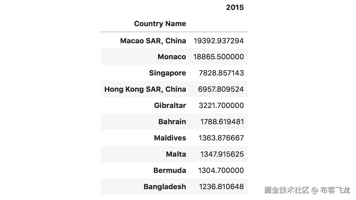
![Figure 1.68: Sorting in descending order](https://p6-xtjj-sign.byteimg.com/tos-cn-i-73owjymdk6/2e25ddd1b5ff45be953b88d83ab5f1c6~tplv-73owjymdk6-jj-mark-v1:0:0:0:0:5o6Y6YeR5oqA5pyv56S-5Yy6IEAg5biD5a6i6aOe6b6Z:q75.awebp?rk3s=f64ab15b&x-expires=1773365502&x-signature=ClMWQC0a3rmPZhcVPwAh8MIgrgc%3D)

###### 图 1.68:按降序排序

**重塑**

11. As we mentioned before, reshaping data with pandas can be a very complex task, so we'll only do an easier reshape. We want to get DataFrames where the columns are country codes and the only row is the year 2015. Since we only have one 2015 label, we need to duplicate it as many times as our dataset length. This will lead to every value receiving the 2015 row index:

```py
# reshaping to 2015 as row and country codes as columns
dataset_2015 = dataset[["Country Code", "2015"]]
dataset_2015.pivot(index=["2015"] * len(dataset_2015), columns="Country Code", values="2015")
```

前面代码的输出如下:

![Figure 1.69: Reshaping the dataset into a single row for the values of 2015](https://p6-xtjj-sign.byteimg.com/tos-cn-i-73owjymdk6/798946255a404cdc9b61818baf87cb2d~tplv-73owjymdk6-jj-mark-v1:0:0:0:0:5o6Y6YeR5oqA5pyv56S-5Yy6IEAg5biD5a6i6aOe6b6Z:q75.awebp?rk3s=f64ab15b&x-expires=1773365502&x-signature=Dk96ttAApR%2BU3K1v9K0ZJKuO7as%3D)

图 1.69:对于 2015 年的值，将数据集重塑为单行

你现在已经完成了关于熊猫的主题，这一章到此结束。我们已经了解了帮助您争论和处理数据的基本工具。熊猫本身是一个令人难以置信的强大和大量使用的数据争论和理解工具。

第二章:关于绘图你需要知道的一切

活动 7:员工技能比较

解决方案:

条形图和雷达图非常适合比较多个组的多个变量。
建议回应:条形图对于比较不同员工的技能属性很有帮助，但是对于一个员工来说，不利于获得整体印象。雷达图非常适合比较员工和技能属性的价值。
Suggested response:

条形图:添加标题和标签，使用不同的颜色

雷达图:为不同的员工增加一个标题和不同的颜色

活动 8:二十年来发生的道路事故

解决方案:

建议回应:我们看一下图 2.20，可以看到 2015 年 1、7 月份事故数量已经减少到 100 起。4 月和 10 月发生了大约 300 起事故。
建议回应:如果我们看一下每个月的趋势，也就是过去二十年的 1 月、4 月、7 月和 10 月，我们可以看到 1 月份发生的事故数量有减少的趋势。

设计实践:

选择视觉有问题的人容易看到的颜色和对比度，这样你的绘图就更具包容性。

活动 9:智能手机销售单位

解决方案:

建议回应:如果对比一下三四季度各个厂商的表现，我们得出苹果表现异常出色的结论。与其他制造商相比，2016 年和 2017 年第三季度至第四季度，他们的销售单位都以更高的速度增长。
建议回应:如果我们看一下各个厂商的销量走势，可以看到 2017 年第三季度之后，除了小米以外的所有公司的销量都出现了不一致的情况。如果看小米的表现，2017 年一季度之后一直有上升趋势。

活动 10:不同时间间隔的列车频率

解决方案:

建议回应:如果我们关注前面的直方图，可以清楚的识别出大部分列车在下午 6 点和 8 点到达。
建议响应:如果下午 4-6 点之间的列车数量增加 50 辆，柱状图将如下所示:

Figure 2.45: Frequency of trains increased by 50 between 4-6 pm

图 2.45:下午 4-6 点之间列车班次增加 50

活动 11:确定理想的可视化

解决方案:

首次可视化 : 建议响应:

提出的可视化有多个缺点:首先，饼图应该显示整体关系的一部分，这不是这个任务的情况，因为我们只考虑前 30 个优酷。其次，30 个值太多，无法在饼图中可视化。第三，切片不是按照大小排序的。此外，由于没有指定测量单位，因此很难量化切片。另一方面，在下面的横条图中，更容易看出每个 YouTube 频道的订户数量(百万):

Figure 2.46: Horizontal bar chart showing Top 30 YouTubers

图 2.46:显示前 30 名优酷的水平条形图

第二次可视化 : 建议响应:

这也是使用错误图表类型的一个例子。折线图用于比较没有任何时间关系的不同类别。此外，图例和标签等信息缺失。下图显示了应该如何使用比较条形图表示数据:

Figure 2.47: Comparative bar chart displaying casino data for two days

图 2.47:显示两天赌场数据的比较条形图

第三章:深入 Matplotlib

活动 12:使用线图可视化股票趋势

解决方案:

让我们用一个线形图来可视化股票趋势:

Open the activity12_solution.ipynb Jupyter Notebook from the Lesson03 folder to implement this activity.

导航到该文件的路径，并在命令行终端键入以下内容:jupyter-lab

导入必要的模块，并在 Jupyter 笔记本中进行绘图:

# Import statements
import matplotlib.pyplot as plt
import numpy as np
import pandas as pd
%matplotlib inline

使用熊猫读取数据文件夹中的数据。read_csv()功能将. csv 文件读入数据框 :

# load datasets
google = pd.read_csv('./data/GOOGL_data.csv')
facebook = pd.read_csv('./data/FB_data.csv')
apple = pd.read_csv('./data/AAPL_data.csv')
amazon = pd.read_csv('./data/AMZN_data.csv')
microsoft = pd.read_csv('./data/MSFT_data.csv')

使用 Matplotlib 创建一个折线图，可视化所有五家公司过去五年的收盘价(整个数据序列)。添加标签、标题和图例，使可视化不言自明。使用plt.grid()功能为您的绘图添加网格:

# Create figure
plt.figure(figsize=(16, 8), dpi=300)
# Plot data
plt.plot('date', 'close', data=google, label='Google')
plt.plot('date', 'close', data=facebook, label='Facebook')
plt.plot('date', 'close', data=apple, label='Apple')
plt.plot('date', 'close', data=amazon, label='Amazon')
plt.plot('date', 'close', data=microsoft, label='Microsoft')
# Specify ticks for x and y axis
plt.xticks(np.arange(0, 1260, 40), rotation=70)
plt.yticks(np.arange(0, 1450, 100))
# Add title and label for y-axis
plt.title('Stock trend', fontsize=16)
plt.ylabel('Closing price in $', fontsize=14)
# Add grid
plt.grid()
# Add legend
plt.legend()
# Show plot
plt.show()

活动 13:创建用于电影比较的条形图

解决方案:

让我们创建一个条形图来比较不同电影的评分:

Open the activity13_solution.ipynb Jupyter Notebook from the Lesson03 folder to implement this activity.

导航到该文件的路径，并在命令行终端键入以下内容:jupyter-lab.

导入必要的模块，并在 Jupyter 笔记本中进行绘图。；

# Import statements
import numpy as np
import pandas as pd
import matplotlib.pyplot as plt
%matplotlib inline

用熊猫读取数据文件夹中的数据:

# Load dataset
movie_scores = pd.read_csv('./data/movie_scores.csv')

使用 Matplotlib 创建一个视觉上吸引人的条形图，比较所有五部电影的两个分数。使用电影标题作为 x 轴的标签。对 y 轴刻度使用 20 的间隔百分比，对 5 的间隔使用次要刻度。给绘图添加一个图例和合适的标题:

# Create figure
plt.figure(figsize=(10, 5), dpi=300)
# Create bar plot
pos = np.arange(len(movie_scores['MovieTitle']))
width = 0.3
plt.bar(pos - width / 2, movie_scores['Tomatometer'], width, label='Tomatometer')
plt.bar(pos + width / 2, movie_scores['AudienceScore'], width, label='Audience Score')
# Specify ticks
plt.xticks(pos, rotation=10)
plt.yticks(np.arange(0, 101, 20))
# Get current Axes for setting tick labels and horizontal grid
ax = plt.gca()
# Set tick labels
ax.set_xticklabels(movie_scores['MovieTitle'])
ax.set_yticklabels(['0%', '20%', '40%', '60%', '80%', '100%'])
# Add minor ticks for y-axis in the interval of 5
ax.set_yticks(np.arange(0, 100, 5), minor=True)
# Add major horizontal grid with solid lines
ax.yaxis.grid(which='major')
# Add minor horizontal grid with dashed lines
ax.yaxis.grid(which='minor', linestyle='--')
# Add title
plt.title('Movie comparison')
# Add legend
plt.legend()
# Show plot
plt.show()

有些功能要求您明确指定轴。要获得对当前轴的引用，请使用ax = plt.gca()。对于 x 轴和 y 轴，可以分别使用plt.xticks([xticks])和plt.yticks([yticks])指定刻度。Axes.set_xticklabels([labels])和Axes.set_yticklabels([labels])可用于设置刻度标签。要添加次要的 y 记号，请使用Axes.set_yticks([ticks], minor=True)。要为主要刻度添加水平网格，请使用Axes.yaxis.grid(which='major')，要为次要刻度添加虚线水平网格，请使用Axes.yaxis.grid(which='minor', linestyle='--')。

活动 14:创建堆叠条形图以可视化餐厅表现

解决方案:

让我们创建一个堆叠条形图来可视化餐厅的表现:

Open the activity14_solution.ipynb Jupyter Notebook from the Lesson03 folder to implement this activity.

导航到该文件的路径，并在命令行终端键入以下内容:jupyter-lab.

导入必要的模块，并在 Jupyter 笔记本中进行绘图:

# Import statements
import pandas as sb
import numpy as np
import matplotlib.pyplot as plt
import seaborn as sns
%matplotlib inline

加载数据集:

# Load dataset
bills = sns.load_dataset('tips')

Use the given dataset and create a matrix where the elements contain the sum of the total bills for each day and smokers/non-smokers:

days = ['Thur', 'Fri', 'Sat', 'Sun']
days_range = np.arange(len(days))
smoker = ['Yes', 'No']
bills_by_days = [bills[bills['day'] == day] for day in days]
bills_by_days_smoker = [[bills_by_days[day][bills_by_days[day]['smoker'] == s] for s in smoker] for day in days_range]
total_by_days_smoker = [[bills_by_days_smoker[day][s]['total_bill'].sum() for s in range(len(smoker))] for day in days_range]
totals = np.asarray(total_by_days_smoker)

这里，asarray()函数用于将任何给定的输入转换成数组。

创建一个堆积条形图，将吸烟者和非吸烟者每天的总账单堆积在一起。添加图例、标签和标题:

# Create figure
plt.figure(figsize=(10, 5), dpi=300)
# Create stacked bar plot
plt.bar(days_range, totals[:, 0], label='Smoker')
plt.bar(days_range, totals[:, 1], bottom=totals[:, 0], label='Non-smoker')
# Add legend
plt.legend()
# Add labels and title
plt.xticks(days_range)
ax = plt.gca()
ax.set_xticklabels(days)
ax.yaxis.grid()
plt.ylabel('Daily total sales in $')
plt.title('Restaurant performance')
# Show plot
plt.show()

活动 15:使用堆叠面积图比较智能手机销量

解决方案:

让我们使用堆叠面积图来比较智能手机制造商的销售单位:

Open the activity15_solution.ipynb Jupyter Notebook from the Lesson03 folder to implement this activity.

导航到该文件的路径，并在命令行终端键入以下内容:jupyter-lab.

导入必要的模块，并在 Jupyter 笔记本中进行绘图:

# Import statements
import pandas as pd
import numpy as np
import matplotlib.pyplot as plt
%matplotlib inline

用熊猫读取数据文件夹中的数据:

# Load dataset
sales = pd.read_csv('./data/smartphone_sales.csv')

创建一个视觉上吸引人的堆叠面积图。添加图例、标签和标题:

# Create figure
plt.figure(figsize=(10, 6), dpi=300)
# Create stacked area chart
labels = sales.columns[1:]
plt.stackplot('Quarter', 'Apple', 'Samsung', 'Huawei', 'Xiaomi', 'OPPO', data=sales, labels=labels)
# Add legend
plt.legend()
# Add labels and title
plt.xlabel('Quarters')
plt.ylabel('Sales units in thousands')
plt.title('Smartphone sales units')
# Show plot
plt.show()

活动 16:使用直方图和箱线图来可视化智商

解决方案:

让我们使用直方图和箱线图来可视化不同群体的智商:

Open the activity16_solution.ipynb Jupyter Notebook from the Lesson03 folder to implement this activity.

导航到该文件的路径，并在命令行终端键入以下内容:jupyter-lab.

导入必要的模块，并在 Jupyter 笔记本中进行绘图:

# Import statements
import numpy as np
import matplotlib.pyplot as plt
%matplotlib inline

使用以下代码生成智商分数样本:

# IQ samples
iq_scores = [126,  89,  90, 101, 102,  74,  93, 101,  66, 120, 108,  97,  98, 105, 119,  92, 113,  81, 104, 108,  83, 102, 105, 111, 102, 107, 103,  89,  89, 110,  71, 110, 120,  85, 111,  83, 122, 120, 102, 84, 118, 100, 100, 114,  81, 109,  69,  97,  95, 106, 116, 109, 114,  98,  90,  92,  98,  91,  81,  85,  86, 102,  93, 112,  76, 89, 110,  75, 100,  90,  96,  94, 107, 108,  95,  96,  96, 114, 93,  95, 117, 141, 115,  95,  86, 100, 121, 103,  66,  99,  96, 111, 110, 105, 110, 91, 112, 102, 112,  75]

为给定的智商分数绘制一个包含 10 个面元的直方图。智商分数呈正态分布，平均值为 100，标准差为 15。将平均值可视化为垂直的红色实线，用垂直虚线表示标准偏差。添加标签和标题:

# Create figure
plt.figure(figsize=(6, 4), dpi=150)
# Create histogram
plt.hist(iq_scores, bins=10)
plt.axvline(x=100, color='r')
plt.axvline(x=115, color='r', linestyle= '--')
plt.axvline(x=85, color='r', linestyle= '--')
# Add labels and title
plt.xlabel('IQ score')
plt.ylabel('Frequency')
plt.title('IQ scores for a test group of a hundred adults')
# Show plot
plt.show()

创建一个方框图来可视化相同的智商分数。添加标签和标题:

# Create figure
plt.figure(figsize=(6, 4), dpi=150)
# Create histogram
plt.boxplot(iq_scores)
# Add labels and title
ax = plt.gca()
ax.set_xticklabels(['Test group'])
plt.ylabel('IQ score')
plt.title('IQ scores for a test group of a hundred adults')
# Show plot
plt.show()

以下是不同测试组的智商分数:

group_a = [118, 103, 125, 107, 111,  96, 104,  97,  96, 114,  96,  75, 114,
       107,  87, 117, 117, 114, 117, 112, 107, 133,  94,  91, 118, 110,
       117,  86, 143,  83, 106,  86,  98, 126, 109,  91, 112, 120, 108,
       111, 107,  98,  89, 113, 117,  81, 113, 112,  84, 115,  96,  93,
       128, 115, 138, 121,  87, 112, 110,  79, 100,  84, 115,  93, 108,
       130, 107, 106, 106, 101, 117,  93,  94, 103, 112,  98, 103,  70,
       139,  94, 110, 105, 122,  94,  94, 105, 129, 110, 112,  97, 109,
       121, 106, 118, 131,  88, 122, 125,  93,  78]
group_b = [126,  89,  90, 101, 102,  74,  93, 101,  66, 120, 108,  97,  98,
            105, 119,  92, 113,  81, 104, 108,  83, 102, 105, 111, 102, 107,
            103,  89,  89, 110,  71, 110, 120,  85, 111,  83, 122, 120, 102,
            84, 118, 100, 100, 114,  81, 109,  69,  97,  95, 106, 116, 109,
            114,  98,  90,  92,  98,  91,  81,  85,  86, 102,  93, 112,  76,
            89, 110,  75, 100,  90,  96,  94, 107, 108,  95,  96,  96, 114,
            93,  95, 117, 141, 115,  95,  86, 100, 121, 103,  66,  99,  96,
            111, 110, 105, 110,  91, 112, 102, 112,  75]
group_c = [108,  89, 114, 116, 126, 104, 113,  96,  69, 121, 109, 102, 107,
       122, 104, 107, 108, 137, 107, 116,  98, 132, 108, 114,  82,  93,
        89,  90,  86,  91,  99,  98,  83,  93, 114,  96,  95, 113, 103,
        81, 107,  85, 116,  85, 107, 125, 126, 123, 122, 124, 115, 114,
        93,  93, 114, 107, 107,  84, 131,  91, 108, 127, 112, 106, 115,
        82,  90, 117, 108, 115, 113, 108, 104, 103,  90, 110, 114,  92,
       101,  72, 109,  94, 122,  90, 102,  86, 119, 103, 110,  96,  90,
       110,  96,  69,  85, 102,  69,  96, 101,  90]
group_d = [ 93,  99,  91, 110,  80, 113, 111, 115,  98,  74,  96,  80,  83,
       102,  60,  91,  82,  90,  97, 101,  89,  89, 117,  91, 104, 104,
       102, 128, 106, 111,  79,  92,  97, 101, 106, 110,  93,  93, 106,
       108,  85,  83, 108,  94,  79,  87, 113, 112, 111, 111,  79, 116,
       104,  84, 116, 111, 103, 103, 112,  68,  54,  80,  86, 119,  81,
        84,  91,  96, 116, 125,  99,  58, 102,  77,  98, 100,  90, 106,
       109, 114, 102, 102, 112, 103,  98,  96,  85,  97, 110, 131,  92,
        79, 115, 122,  95, 105,  74,  85,  85,  95]

为不同测试组的每个智商分数创建一个方框图。添加标签和标题:

# Create figure
plt.figure(figsize=(6, 4), dpi=150)
# Create histogram
plt.boxplot([group_a, group_b, group_c, group_d])
# Add labels and title
ax = plt.gca()
ax.set_xticklabels(['Group A', 'Group B', 'Group C', 'Group D'])
plt.ylabel('IQ score')
plt.title('IQ scores for different test groups')
# Show plot
plt.show()

活动 17:使用散点图来可视化各种动物之间的相关性

解决方案:

让我们借助散点图来可视化各种动物之间的相关性:

Open the activity17_solution.ipynb Jupyter Notebook from the Lesson03 folder to implement this activity.

导航到该文件的路径，并在命令行终端键入以下内容:jupyter-lab.

导入必要的模块，并在 Jupyter 笔记本中进行绘图:

# Import statements
import pandas as pd
import numpy as np
import matplotlib.pyplot as plt
%matplotlib inline

用熊猫读取数据文件夹中的数据:

# Load dataset 
data = pd.read_csv('./data/anage_data.csv')

给定的数据集不完整。过滤数据，这样你最终得到的样本就包含了一个体重和最长寿命。根据动物种类对数据进行分类。这里，isfinite()函数检查给定元素的有限性:

# Preprocessing
longevity = 'Maximum longevity (yrs)'
mass = 'Body mass (g)'
data = data[np.isfinite(data[longevity]) & np.isfinite(data[mass])]
# Sort according to class
amphibia = data[data['Class'] == 'Amphibia']
aves = data[data['Class'] == 'Aves']
mammalia = data[data['Class'] == 'Mammalia']
reptilia = data[data['Class'] == 'Reptilia']

创建散点图，可视化体重和最大寿命之间的相关性。根据数据样本的类别，使用不同的颜色对数据样本进行分组。添加图例、标签和标题。x 轴和 y 轴都使用对数刻度:

# Create figure
plt.figure(figsize=(10, 6), dpi=300)
# Create scatter plot
plt.scatter(amphibia[mass], amphibia[longevity], label='Amphibia')
plt.scatter(aves[mass], aves[longevity], label='Aves')
plt.scatter(mammalia[mass], mammalia[longevity], label='Mammalia')
plt.scatter(reptilia[mass], reptilia[longevity], label='Reptilia')
# Add legend
plt.legend()
# Log scale
ax = plt.gca()
ax.set_xscale('log')
ax.set_yscale('log')
# Add labels
plt.xlabel('Body mass in grams')
plt.ylabel('Maximum longevity in years')
# Show plot
plt.show()

活动 18:创建带有边缘直方图的散点图

解决方案:

Open the activity18_solution.ipynb Jupyter Notebook from the Lesson03 folder to implement this activity.

导航到该文件的路径，并在命令行终端键入以下内容:jupyter-lab.

导入必要的模块，并在 Jupyter 笔记本中进行绘图:

# Import statements
import pandas as pd
import numpy as np
import matplotlib.pyplot as plt
%matplotlib inline

用熊猫读取数据文件夹中的数据:

# Load dataset
data = pd.read_csv('./data/anage_data.csv')

给定的数据集不完整。过滤数据，这样你最终得到的样本就包含了一个体重和最长寿命。选择所有aves类且体重小于 20，000 的样本:

# Preprocessing
longevity = 'Maximum longevity (yrs)'
mass = 'Body mass (g)'
data = data[np.isfinite(data[longevity]) & np.isfinite(data[mass])]
# Sort according to class
aves = data[data['Class'] == 'Aves']
aves = data[data[mass] < 20000]

创建具有受约束布局的图形。创建一个 4x4 大小的网格像素。创建大小为 3x3 的散点图和大小为 1x3 和 3x1 的边缘直方图。添加标签和图形标题:

# Create figure
fig = plt.figure(figsize=(8, 8), dpi=150, constrained_layout=True)
# Create gridspec
gs = fig.add_gridspec(4, 4)
# Specify subplots
histx_ax = fig.add_subplot(gs[0, :-1])
histy_ax = fig.add_subplot(gs[1:, -1])
scatter_ax = fig.add_subplot(gs[1:, :-1])
# Create plots
scatter_ax.scatter(aves[mass], aves[longevity])
histx_ax.hist(aves[mass], bins=20, density=True)
histx_ax.set_xticks([])
histy_ax.hist(aves[longevity], bins=20, density=True, orientation='horizontal')
histy_ax.set_yticks([])
# Add labels and title
plt.xlabel('Body mass in grams')
plt.ylabel('Maximum longevity in years')
fig.suptitle('Scatter plot with marginal histograms')
# Show plot
plt.show()

活动 19:在网格中绘制多个图像

解决方案:

Open the activity19_solution.ipynb Jupyter Notebook from the Lesson03 folder to implement this activity.

导航到该文件的路径，并在命令行终端键入以下内容:jupyter-lab.

导入必要的模块，并在 Jupyter 笔记本中进行绘图:

# Import statements
import os
import numpy as np
import matplotlib.pyplot as plt
import matplotlib.image as mpimg
%matplotlib inline

从数据文件夹加载所有四个图像:

# Load images
img_filenames = os.listdir('data')
imgs = [mpimg.imread(os.path.join('data', img_filename)) for img_filename in img_filenames]

在 2x2 网格中可视化图像。移除轴并给每个图像一个标签:

# Create subplot
fig, axes = plt.subplots(2, 2)
fig.figsize = (6, 6)
fig.dpi = 150
axes = axes.ravel()
# Specify labels
labels = ['coast', 'beach', 'building', 'city at night']
# Plot images
for i in range(len(imgs)):
    axes[i].imshow(imgs[i])
    axes[i].set_xticks([])
    axes[i].set_yticks([])
    axes[i].set_xlabel(labels[i])

第 4 章:使用 Seaborn 简化可视化

活动 20:使用箱线图比较不同测试组的智商得分

解决方案:

让我们使用 Seaborn 库来比较不同测试组的智商得分:

从Lesson04文件夹打开activity20_solution.ipynb Jupyter 笔记本，执行本活动。导航到该文件的路径，并在命令行终端键入以下内容:jupyter-lab。

导入必要的模块，并在 Jupyter 笔记本中进行绘图。

%matplotlib inline
import numpy as np
import pandas as pd
import matplotlib.pyplot as plt
import seaborn as sns

使用熊猫read_csv()功能读取数据文件夹中的数据:
```
mydata = pd.read_csv("./data/scores.csv")
```
访问列中每个测试组的数据。使用tolist()方法将其转换为列表。一旦每个测试组的数据被转换成一个列表，将这个列表分配给每个测试组的变量:
```
group_a = mydata[mydata.columns[0]].tolist()
group_b = mydata[mydata.columns[1]].tolist()
group_c = mydata[mydata.columns[2]].tolist()
group_d = mydata[mydata.columns[3]].tolist()
```
Print the variables of each group to check whether the data inside it is converted into a list. This can be done with the help of the print() function:
```
print(group_a)
```
A 组的数据值如下图所示:

图 4.35:A 组的值
```
print(group_b)
```
乙组的数据值如下图所示:

图 4.36:乙组的数值
```
print(group_c)
```
C 组的数据值如下图所示:

图 4.37:C 组的值
```
print(group_d)
```
D 组的数据值如下图所示:

图 4.38:D 组的值

一旦我们有了每个测试组的数据，我们就需要从这个给定的数据构建一个数据框架。这可以借助熊猫提供的pd.DataFrame()功能来完成。

data = pd.DataFrame({'Groups': ['Group A'] * len(group_a) + ['Group B'] * len(group_b) + ['Group C'] * len(group_c) + ['Group D'] * len(group_d),
                     'IQ score': group_a + group_b + group_c + group_d})

Now, since we have the DataFrame, we need to create a box plot using the boxplot() function that's provided by Seaborn. Within this function, we need to specify the titles for both the axes along with the DataFrame we are using. The title for the x-axis would be Groups and the title for the y-axis would be IQ score. As far as the DataFrame is concerned, we will pass data as a parameter. Here, data is the DataFrame that we obtained from the previous step.
```
plt.figure(dpi=150)
# Set style
sns.set_style('whitegrid')
# Create boxplot
sns.boxplot('Groups', 'IQ score', data=data)
# Despine
sns.despine(left=True, right=True, top=True)
# Add title
plt.title('IQ scores for different test groups')
# Show plot
plt.show() 
```
despine()功能有助于从图中移除顶部和右侧的刺。这里，我们还切除了左侧脊柱。使用title()功能，我们已经为我们的绘图设置了标题。show()功能有助于可视化绘图。

从图 4.8 中，我们可以得出结论，通过使用方框图，A 组的智商得分优于其他组。

活动 21:使用热图寻找航班乘客数据中的模式

解决方案:

让我们借助热图找出航班乘客数据中的模式:

从Lesson04文件夹打开activity21_solution.ipynb Jupyter 笔记本，执行本活动。导航到该文件的路径，并在命令行终端键入以下内容:jupyter-lab。

导入必要的模块，并在 Jupyter 笔记本中进行绘图:

%matplotlib inline
import numpy as np
import pandas as pd
import matplotlib.pyplot as plt
import seaborn as sns

使用熊猫的read_csv()功能读取数据文件夹中的数据:
```
mydata = pd.read_csv("./data/flight_details.csv")
```
现在，我们可以使用pivot()函数为我们的数据框提供有意义的行和列标签:
```
data = mydata.pivot("Months", "Years", "Passengers")
```
使用 Seaborn 库的heatmap()功能来可视化这些数据。在这个函数中，我们传递数据帧和颜色映射等参数。由于我们从前面的代码中获得了数据，我们将把它作为heatmap()函数中的数据框传递。此外，我们将创建自己的颜色映射，并将其作为第二个参数传递给这个函数。
```
sns.set()
plt.figure(dpi=150)
sns.heatmap(data, cmap=sns.light_palette("orange", as_cmap=True, reverse=True))
plt.title("Flight Passengers from 2001 to 2012")
plt.show()
```

从图 4.23 中，我们可以得出结论，2012 年 7 月和 8 月的航班乘客数量最高。

活动 22:重温电影对比

解决方案:

让我们使用 Seaborn library 提供的条形图来比较五部不同电影的电影评分:

从Lesson04文件夹打开activity22_solution.ipynb Jupyter 笔记本，执行本活动。导航到该文件的路径，并在命令行终端键入以下内容:jupyter-lab。

导入必要的模块，并在 Jupyter 笔记本中进行绘图:

%matplotlib inline
import numpy as np
import pandas as pd
import matplotlib.pyplot as plt
import seaborn as sns

使用熊猫的read_csv()功能读取数据文件夹中的数据:
```
mydata = pd.read_csv("./data/movie_scores.csv")
```

从这个给定的数据构造一个数据帧。这可以借助熊猫提供的pd.DataFrame()功能来完成。下面的代码让我们对此有了更好的了解:

movie_scores = pd.DataFrame({"Movie Title": list(mydata["MovieTitle"]) * 2,
                "Score": list(mydata["AudienceScore"]) + list(mydata["Tomatometer"]),
                "Type": ["Audience Score"] * len(mydata["AudienceScore"]) + ["Tomatometer"] * len(mydata["Tomatometer"])})

Make use of the barplot() function provided by Seaborn. Provide Movies and Scores as parameters so that their data is displayed on both axes. Provide Type as hue, on the basis of which the comparison needs to be made. The last parameter needs a DataFrame as input. Thus, we provide the movie_scores DataFrame, which we obtained from the previous step.

下面的代码对此有更好的理解:
```
sns.set()
plt.figure(figsize=(10, 5), dpi=300)
# Create bar plot
ax = sns.barplot("Movie Title", "Score", hue="Type", data=movie_scores)
plt.xticks(rotation=10)
# Add title
plt.title("Movies Scores comparison")
plt.xlabel("Movies")
plt.ylabel("Scores")
# Show plot
plt.show()
```

我们比较了 AudienceScore 和 Tomatometer 对 5 部不同电影的评分，并得出结论，电影《T0》和《火星人》的评分相匹配。

活动 23:使用小提琴图比较不同测试组的智商得分

解决方案:

让我们使用 Seaborn 库来比较不同测试组的智商得分:

从Lesson04文件夹打开activity23_solution.ipynb Jupyter 笔记本，执行本活动。导航到该文件的路径，并在命令行终端键入以下内容:jupyter-lab。

导入必要的模块，并在 Jupyter 笔记本中进行绘图:

%matplotlib inline
import numpy as np
import pandas as pd
import matplotlib.pyplot as plt
import seaborn as sns

使用熊猫的read_csv()功能读取数据文件夹中的数据:
```
mydata = pd.read_csv("./data/scores.csv")
```
访问列中每个测试组的数据。使用tolist()方法将其转换为列表。一旦每个测试组的数据被转换成一个列表，将这个列表分配给每个测试组的变量。
```
group_a = mydata[mydata.columns[0]].tolist()
group_b = mydata[mydata.columns[1]].tolist()
group_c = mydata[mydata.columns[2]].tolist()
group_d = mydata[mydata.columns[3]].tolist()
```
Print the variables of each group to check whether the data inside it has been converted into a list. This can be done with the help of the print() function:
```
print(group_a)
```
图 4.39:A 组的值
```
print(group_b)
```
图 4.40:乙组的数值
```
print(group_c)
```
图 4.41:C 组的值
```
print(group_d)
```
图 4.42:D 组的值

一旦我们获得了每个测试组的数据，我们需要从这个给定的数据中构建一个数据框架。这可以通过熊猫提供的pd.DataFrame()功能来实现。

data = pd.DataFrame({'Groups': ['Group A'] * len(group_a) + ['Group B'] * len(group_b) + ['Group C'] * len(group_c) + ['Group D'] * len(group_d),
                     'IQ score': group_a + group_b + group_c + group_d})

Now, since we have the DataFrame, we need to create a violin plot using the violinplot() function that's provided by Seaborn. Within this function, we need to specify the titles for both the axes along with the DataFrame we are using. The title for the x-axis will be Groups and the title for the y-axis will be IQ score. As far as the DataFrame is concerned, we will pass data as a parameter. Here, data is the DataFrame that we obtained from the previous step.
```
plt.figure(dpi=150)
# Set style
sns.set_style('whitegrid')
# Create boxplot
sns.violinplot('Groups', 'IQ score', data=data)
# Despine
sns.despine(left=True, right=True, top=True)
# Add title
plt.title('IQ scores for different test groups')
# Show plot
plt.show() 
```
despine()功能有助于从图中移除顶部和右侧的刺。这里，我们还切除了左侧脊柱。使用title()功能，我们已经为我们的绘图设置了标题。show()功能有助于可视化绘图。

我们可以得出结论，A 组的智商得分比其他组好。

活动 24:排名前 30 的 YouTube 频道

解决方案:

让我们通过使用由 Seaborn 图书馆提供的FacetGrid()功能来可视化前 30 个 YouTube 频道的订户总数和总浏览量:

从Lesson04文件夹打开activity24_solution.ipynb Jupyter 笔记本，执行本活动。导航到该文件的路径，并在命令行终端键入以下内容:jupyter-lab。

导入必要的模块，并在 Jupyter 笔记本中进行绘图:

%matplotlib inline
import numpy as np
import pandas as pd
import matplotlib.pyplot as plt
import seaborn as sns

使用熊猫的read_csv()功能读取数据文件夹中的数据:
```
mydata = pd.read_csv("./data/youtube.csv")
```
访问列中每个测试组的数据。使用tolist()方法将其转换为列表。一旦每个测试组的数据被转换成一个列表，将这个列表分配给每个测试组的变量。
```
channels = mydata[mydata.columns[0]].tolist()
subs = mydata[mydata.columns[1]].tolist()
views = mydata[mydata.columns[2]].tolist()
```
Print the variables of each group to check whether the data inside it has been converted into a list. This can be done with the help of the print() function:
```
print(channels)
```
图 4.43:YouTube 频道列表
```
print(subs)
```
图 4.44:每个 YouTube 频道的订户列表
```
print(views)
```
图 4.45:每个 YouTube 频道的视图列表
一旦我们获得了channels、subs和views的数据，我们需要从这个给定的数据构建一个数据框架。这可以通过熊猫提供的pd.DataFrame()功能来实现。
```
data = pd.DataFrame({'YouTube Channels': channels + channels, 'Subscribers in millions': subs + views, 'Type': ['Subscribers'] * len(subs) + ['Views'] * len(views)})
```
现在，既然我们有了数据框架，我们需要使用 Seaborn 提供的FacetGrid()函数创建一个 FacetGrid。这里，data是我们从上一步获得的数据帧。
```
sns.set()
g = sns.FacetGrid(data, col='Type', hue='Type', sharex=False, height=8)
g.map(sns.barplot, 'Subscribers in millions', 'YouTube Channels')
plt.show()
```

我们可以得出结论，PewDiePie 的 YouTube 频道拥有最高的订户数量，而 T-Series 拥有最高的浏览量。

活动 25:线性回归

解决方案:

让我们通过使用由 Seaborn 库提供的regplot()函数来可视化回归图中最大寿命和体重之间的线性关系:

从Lesson04文件夹打开activity25_solution.ipynb Jupyter 笔记本，执行本活动。导航到该文件的路径，并在命令行终端键入以下内容:jupyter-lab。

导入必要的模块，并在 Jupyter 笔记本中进行绘图:

%matplotlib inline
import numpy as np
import pandas as pd
import matplotlib.pyplot as plt
import seaborn as sns

使用熊猫的read_csv()功能读取数据文件夹中的数据:
```
mydata = pd.read_csv("./data/anage_data.csv")
```

过滤数据，这样你最终得到的样本就包含了一个体重和最长寿命。只考虑Mammalia级和体重低于 20 万的样本。这个预处理可以在下面的代码中看到:

longevity = 'Maximum longevity (yrs)'
mass = 'Body mass (g)'
data = mydata[mydata['Class'] == 'Mammalia']
data = data[np.isfinite(data[longevity]) & np.isfinite(data[mass]) & (data[mass] < 200000)]

预处理完成后，我们需要使用 Seaborn 库提供的regplot()函数绘制数据。在下面的代码中，我们在regplot()函数中提供了三个参数。前两个参数为mass和longevity，其中 x 轴显示体重数据，y 轴显示最大寿命数据。在第三个参数中，我们需要提供一个名为data的数据帧，它是我们从上一步中获得的:
```
# Create figure
sns.set()
plt.figure(figsize=(10, 6), dpi=300)
# Create scatter plot
sns.regplot(mass, longevity, data=data)
# Show plot
plt.show()
```

我们可以得出结论，Mammalia级的体重和最大寿命之间存在线性关系。

活动 26:重新审视水的使用

解决方案:

让我们通过使用树图来可视化用水量，树图可以在 Squarify 库的帮助下创建:

从Lesson 04文件夹打开activity26_solution.ipynb Jupyter 笔记本，执行本活动。导航到该文件的路径，并在命令行终端键入以下内容:jupyter-lab。

导入必要的模块，并在 Jupyter 笔记本中进行绘图:

%matplotlib inline
import numpy as np
import pandas as pd
import matplotlib.pyplot as plt
import seaborn as sns
import squarify

使用熊猫的read_csv()功能读取数据文件夹中的数据:
```
mydata = pd.read_csv("./data/water_usage.csv")
```
通过访问前面数据集中的每一列来创建标签列表。这里，astype('str')函数用于将提取的数据转换为类型字符串。
```
# Create figure
plt.figure(dpi=200)
# Create tree map
labels = mydata['Usage'] + ' (' + mydata['Percentage'].astype('str') + '%)'
```
为了创建给定数据的树形图可视化，我们使用了squarify库的plot()功能。这个函数有三个参数。第一个参数是所有百分比的列表，第二个参数是所有标签的列表，这是我们在上一步中得到的。第三个参数是可以使用 Seaborn 库的light_pallete()功能创建的颜色。
```
squarify.plot(sizes=mydata['Percentage'], label=labels, color=sns.light_palette('green', mydata.shape[0]))
plt.axis('off')
# Add title
plt.title('Water usage')
# Show plot
plt.show()
```

第 5 章:绘制地理空间数据

活动 27:在地图上绘制地理空间数据

解决方案:

让我们在地图上绘制地理空间数据，并找到欧洲人口超过 10 万的城市的人口密集区:

从Lesson05文件夹打开activity27.ipynb Jupyter 笔记本，执行本活动。

在开始处理数据之前，我们需要导入依赖项:

# importing the necessary dependencies
import numpy as np
import pandas as pd
import geoplotlib

Load the dataset using pandas:
```
#loading the Dataset (make sure to have the dataset downloaded)
Dataset = pd.read_csv('./data/world_cities_pop.csv', dtype = {'Region': np.str})
```
注意

如果我们导入数据集时没有将Region列的dtype定义为String，我们将收到一条警告，告诉我们它具有混合数据类型。我们可以通过显式定义此列中值的类型来消除此警告，这可以通过使用dtype参数来实现。
To see the dtype of each column, we can use the dtypes attribute of a DataFrame:
```
# looking at the data types of each column
Dataset.dtypes
```
下图显示了前面代码的输出:

图 5.18:数据集每一列的数据类型

注意

在这里，我们可以看到每一列的数据类型。由于String类型不是一个原始数据类型，它被显示为一个对象。
We use the head() method of pandas DataFrames to display the first five entries:
```
# showing the first 5 entries of the dataset
dataset.head()
```
下图显示了前面代码的输出:

图 5.19:数据集的前五个条目
大多数数据集不会是您想要的格式。其中一些可能将它们的Latitude和Longitude值隐藏在不同的列中。这就是需要第一章数据可视化和数据探索的数据角力技巧的地方。对于给定的数据集，转换很简单——我们只需要将Latitude和Longitude列映射到lat和lon列，这是通过赋值完成的:
```
# mapping Latitude to lat and Longitude to lon
dataset['lat'] = dataset['Latitude']
dataset['lon'] = dataset['Longitude']
```
Our dataset is now ready for the first plotting. We'll use a DotDensityLayer here, which is a good way to start and see all of our data points:
```
# plotting the whole dataset with dots
geoplotlib.dot(dataset)
geoplotlib.show()
```
下图显示了前面代码的输出:

图 5.20:所有城市的点密度可视化
Before we start breaking down our data to get a better and more workable dataset, we want to understand the outlines of our full data. We'll do this by displaying the number of countries and the number of cities that our dataset holds:
```
# amount of countries and cities
print(len(dataset.groupby(['Country'])), 'Countries')
print(len(dataset), 'Cities')
```
下图显示了前面代码的输出:

图 5.21:按国家和城市分组
To see each grouped element on its own, we use the size() method, which returns a Series object:
```
# amount of cities per country (first 20 entries)
dataset.groupby(['Country']).size().head(20)
```
下图显示了前面代码的输出:

图 5.22:每个国家的城市数量
We also want to display the average amount of cities per country. Aggregation is an important concept in pandas that helps us in achieving this:

```py

# average num of cities per country
dataset.groupby(['Country']).size().agg('mean')
```

下图显示了前面代码的输出:

![Figure 5.23: Average amount of cities per country ](https://p6-xtjj-sign.byteimg.com/tos-cn-i-73owjymdk6/d47db5911e5d4bd4b268313be22e2bb8~tplv-73owjymdk6-jj-mark-v1:0:0:0:0:5o6Y6YeR5oqA5pyv56S-5Yy6IEAg5biD5a6i6aOe6b6Z:q75.awebp?rk3s=f64ab15b&x-expires=1773365502&x-signature=wefBL%2Fse%2BkFrN1IW4diU5zaCIAA%3D)

###### 图 5.23:每个国家的平均城市数量

11. We now want to reduce the amount of data we are working with. One approach would be to remove all cities that don't have a population value:

#### 注意

分解和过滤你的数据是获得好的洞察力的最重要的方面之一。杂乱的可视化可以隐藏信息。

```py
# filter for countries with a population entry (Population > 0)
dataset_with_pop = dataset[(dataset['Population'] > 0)]
print('Full dataset:', len(dataset))
print('Cities with population information:', len(dataset_with_pop))
```

下图显示了前面代码的输出:

![Figure 5.24: Cities with population information ](https://p6-xtjj-sign.byteimg.com/tos-cn-i-73owjymdk6/e307532bacc44e4b8daad9f14376ad52~tplv-73owjymdk6-jj-mark-v1:0:0:0:0:5o6Y6YeR5oqA5pyv56S-5Yy6IEAg5biD5a6i6aOe6b6Z:q75.awebp?rk3s=f64ab15b&x-expires=1773365502&x-signature=7S74NM7hauYgjxmHZE1eh89Bn18%3D)

###### 图 5.24:有人口信息的城市

12. Displaying the first five items from the new dataset gives us a basic indication of what values will be present in the Population column:

```py
# displaying the first 5 items from dataset_with_pop
dataset_with_pop.head()
```

下图显示了前面代码的输出:

![Figure 5.25: First five items of the reduced dataset ](https://p6-xtjj-sign.byteimg.com/tos-cn-i-73owjymdk6/b1862ba29c8e4565a11d337e55417757~tplv-73owjymdk6-jj-mark-v1:0:0:0:0:5o6Y6YeR5oqA5pyv56S-5Yy6IEAg5biD5a6i6aOe6b6Z:q75.awebp?rk3s=f64ab15b&x-expires=1773365502&x-signature=UvEUf5e0nyLn9de8OkJ1j%2FpyfdE%3D)

###### 图 5.25:缩减数据集的前五项

13. Now. we can take a look at our reduced dataset with the help of a dot-densityplot:

```py
# showing all cities with a defined population with a dot density plot
geoplotlib.dot(dataset_with_pop)
geoplotlib.show()
```

在新的点图中，我们已经可以感受到清晰度方面的一些改进。我们的地图上仍然有太多的点。给定活动定义，我们可以通过只查看人口超过 10 万的城市来进一步过滤数据集。

14. To further filter our dataset, we can use the same approach that we used previously:

```py
# dataset with cities with population of >= 100k
dataset_100k = dataset_with_pop[(dataset_with_pop['Population'] >= 100_000)]
print('Cities with a population of 100k or more:', len(dataset_100k))
```

下图显示了前面代码的输出:

![Figure 5.26: Cities with a population of 100k or more ](https://p6-xtjj-sign.byteimg.com/tos-cn-i-73owjymdk6/65c77ff1705743d18c7c972777c20799~tplv-73owjymdk6-jj-mark-v1:0:0:0:0:5o6Y6YeR5oqA5pyv56S-5Yy6IEAg5biD5a6i6aOe6b6Z:q75.awebp?rk3s=f64ab15b&x-expires=1773365502&x-signature=mPBQScmeH2yqk6vd%2FD%2FIc59CuJA%3D)

###### 图 5.26:人口超过 10 万的城市

15. In addition to just plotting our 100k dataset, we also want to fix our viewport to a specific bounding box. Since our data is spread across the world, we can use the in-built WORLD constant of the BoundingBox class:

```py
# displaying all cities >= 100k population with a fixed bounding box (WORLD) in a dot density plot
from geoplotlib.utils import BoundingBox
geoplotlib.dot(dataset_100k)
geoplotlib.set_bbox(BoundingBox.WORLD)
geoplotlib.show()
```

下图显示了前面代码的输出:

![Figure 5.27: Dot-density visualization of cities with a population of 100k or more ](https://p6-xtjj-sign.byteimg.com/tos-cn-i-73owjymdk6/cf956aff69cb444f93a4aa0eff0000fc~tplv-73owjymdk6-jj-mark-v1:0:0:0:0:5o6Y6YeR5oqA5pyv56S-5Yy6IEAg5biD5a6i6aOe6b6Z:q75.awebp?rk3s=f64ab15b&x-expires=1773365502&x-signature=mDn41PFWq%2BiORXDenA5YoC1%2BPcs%3D)

###### 图 5.27:人口超过 10 万的城市的点密度可视化

16. Comparing it with the previous plots, it gives us a better view on where large amounts of cities are with a population of more than 100k. We now want to find the areas of these cities that are the most densely packed. As we've seen in the previous exercise, Voronoi is convenient for such insights:

```py
# using filled voronoi to find dense areas
geoplotlib.voronoi(dataset_100k, cmap='hot_r', max_area=1e3, alpha=255)
geoplotlib.show()
```

结果可视化正是我们所寻找的。在沃罗诺伊绘图中，我们可以看到明显的倾向。德国、英国、尼日利亚、印度、日本、爪哇、美国东海岸和巴西脱颖而出。我们现在可以过滤我们的数据，只看那些国家，找到最适合的。

#### 注意

您也可以使用`ColorMap`类创建自定义颜色映射渐变。

17. The last step is to reduce our dataset to countries in Europe, such as Germany and Great Britain. We can use operators when supplying conditions to filter our data. This operator will allow us to filter for Germany and Great Britain at the same time:

```py
# filter 100k dataset for cities in Germany and GB
dataset_europe = dataset_100k[(dataset_100k['Country'] == 'de') | (dataset_100k['Country'] == 'gb')]
print('Cities in Germany or GB with population >= 100k:', len(dataset_europe))
```

![Figure 5.28: Cities in Germany and Great Britain with a population of 100K or more ](https://p6-xtjj-sign.byteimg.com/tos-cn-i-73owjymdk6/08de6b36a01c43b58e1ea682d3cc7f7d~tplv-73owjymdk6-jj-mark-v1:0:0:0:0:5o6Y6YeR5oqA5pyv56S-5Yy6IEAg5biD5a6i6aOe6b6Z:q75.awebp?rk3s=f64ab15b&x-expires=1773365502&x-signature=BFTcsEm%2F26YlSrulJpBUAiTDiGc%3D)

###### 图 5.28:德国和英国人口超过 10 万的城市

18. Using Delaunay triangulation to find the area with the most densely packed cities, we can see one more hotspot. The areas around Cologne, Birmingham, and Manchester really stick out:

```py
#using Delaunay triangulation to find the most densely populated area
geoplotlib.delaunay(dataset_europe, cmap='hot_r')
geoplotlib.show()
```

通过使用`hot_r`彩色地图，我们可以快速获得良好的视觉表现，并使感兴趣的区域突出。

恭喜你！您已经使用 Geoplotlib 完成了第一项活动。我们利用不同的绘图来获得我们需要的信息。在接下来的活动中，我们将查看 Geoplotlib 的更多自定义功能，以更改地图切片提供程序并创建自定义绘制图层。

活动 28:使用自定义图层

解决方案:

让我们创建一个自定义图层**，**将允许我们显示地理空间数据并随着时间的推移对数据点进行动画处理 :

在第一步中，我们只需要pandas进行数据导入:

# importing the necessary dependencies
import pandas as pd

Use the read_csv method of pandas to load the .csv file:
```
# loading the dataset from the csv file
dataset = pd.read_csv('./data/flight_tracking.csv')
```
注意

前面的数据集可以在这里找到:bit.ly/2DyPHwD。
We need to understand the structure of our dataset by looking at the provided features:
```
# displaying the first 5 rows of the dataset
dataset.head()
```
图 5.29:数据集的前五个元素

请记住，地理图书馆需要名称为lat和lon的latitude和longitude列。使用熊猫中提供的rename方法重命名列:

# renaming columns latitude to lat and longitude to lon
dataset = dataset.rename(index=str, columns={"latitude": "lat", "longitude": "lon"})

Taking another look at the first five elements of the dataset, we can now observe that the names of the columns have changed to lat and lon:
```
# displaying the first 5 rows of the dataset
dataset.head()
```
图 5.30:包含 lat 和 lon 列的数据集

Since we want to get a visualization over time in this activity, we need to work with date and time. If we take a closer look at our dataset, it shows us that date and time are separated by two columns.

我们需要使用to_epoch方法将日期和时间合并成一个时间戳。下面的代码可以做到这一点:

# method to convert date and time to an unix timestamp
from datetime import datetime
def to_epoch(date, time):
    try:
        timestamp = round(datetime.strptime('{} {}'.format(date, time), '%Y/%m/%d %H:%M:%S.%f').timestamp())
        return timestamp
    except ValueError:
        return round(datetime.strptime('2017/09/11 17:02:06.418', '%Y/%m/%d %H:%M:%S.%f').timestamp())

使用前面的方法，我们现在可以使用 pandas DataFrame 提供的apply方法创建一个名为timestamp的新列，该列保存 unix 时间戳:

# creating a new column called timestamp with the to_epoch method applied
dataset['timestamp'] = dataset.apply(lambda x: to_epoch(x['date'], x['time']), axis=1)

Taking another look at our dataset, we now have a new column that holds the unix timestamps:
```
# displaying the first 5 rows of the dataset
dataset.head()
```
图 5.31:添加了时间戳列的数据集

由于我们的数据集现在已经准备好与所有必要的列一起使用，我们可以开始编写我们的自定义层了。一旦到达数据集中提供的timestamp，该图层将显示每个点。它将显示几秒钟，然后消失。我们需要跟踪定制层中的当前时间戳。巩固我们在本主题理论部分所学的内容，我们有一个__init__方法来构建我们的定制TrackLayer。

In our draw method, we filter our dataset for all the elements that are in the mentioned time range and use each element of the filtered list to display it on the map with color that's provided by the colorbrewer method.

由于我们的数据集只包含来自特定时间范围的数据，并且我们总是递增时间，所以我们想要检查在当前时间戳之后是否还有任何带有timestamps的元素。如果没有，我们希望将当前时间戳设置为数据集中可用的最早时间戳。下面的代码显示了我们如何创建自定义图层:

# custom layer creation
import geoplotlib
from geoplotlib.layers import BaseLayer
from geoplotlib.core import BatchPainter
from geoplotlib.colors import colorbrewer
from geoplotlib.utils import epoch_to_str, BoundingBox
class TrackLayer(BaseLayer):
    def __init__(self, dataset, bbox=BoundingBox.WORLD):
        self.data = dataset
        self.cmap = colorbrewer(self.data['hex_ident'], alpha=200)
        self.time = self.data['timestamp'].min()
        self.painter = BatchPainter()
        self.view = bbox
    def draw(self, proj, mouse_x, mouse_y, ui_manager):
        self.painter = BatchPainter()
        df = self.data.where((self.data['timestamp'] > self.time) & (self.data['timestamp'] <= self.time + 180))
        for element in set(df['hex_ident']):
            grp = df.where(df['hex_ident'] == element)
            self.painter.set_color(self.cmap[element])
            x, y = proj.lonlat_to_screen(grp['lon'], grp['lat'])
            self.painter.points(x, y, 15, rounded=True)
        self.time += 1
        if self.time > self.data['timestamp'].max():
            self.time = self.data['timestamp'].min()
        self.painter.batch_draw()
        ui_manager.info('Current timestamp: {}'.format(epoch_to_str(self.time)))

    # bounding box that gets used when layer is created
    def bbox(self):
        return self.view

由于我们的数据集只包含来自英国利兹周边地区的数据，因此我们需要定义一个自定义BoundingBox，将我们的视图集中在该地区:

```py

# bounding box for our view on Leeds
from geoplotlib.utils import BoundingBox
leeds_bbox = BoundingBox(north=53.8074, west=-3, south=53.7074 , east=0)
```

11. 地质图书馆有时要求你提供一个DataAccessObject而不是熊猫数据框。Geoplotlib 提供了一种将任何熊猫数据帧转换成DataAccessObject :

```py
# displaying our custom layer using add_layer
from geoplotlib.utils import DataAccessObject
data = DataAccessObject(dataset)
geoplotlib.add_layer(TrackLayer(data, bbox=leeds_bbox))
geoplotlib.show()
```

的便捷方法

恭喜你！您已经使用 Geoplotlib 完成了自定义图层活动。我们已经应用了几个预处理步骤来按照我们想要的方式塑造数据集。我们还编写了一个自定义图层来显示时间空间中的空间数据。我们的自定义层甚至有一个动画级别。这是我们将在下一章详细讨论的内容。

第六章:让事物与 Bokeh 互动

活动 29:使用小部件扩展绘图

解决方案:

从Lesson06文件夹打开activity29_solution.ipynb Jupyter 笔记本，执行本活动。

导入必要的库:

# importing the necessary dependencies
import pandas as pd

同样，我们希望在 Jupyter 笔记本中显示我们的绘图，因此我们必须从 Bokeh 的io界面导入并调用output_notebook方法:
```
# make bokeh display figures inside the notebook
from bokeh.io import output_notebook
output_notebook()
```
下载数据集并移动到本章的数据文件夹后，我们可以导入我们的olympia2016_athletes.csv数据:
```
# loading the Dataset with geoplotlib
dataset = pd.read_csv('./data/olympia2016_athletes.csv')
```
A quick test by calling head on our DataFrame shows us that our data has been successfully loaded:
```
# looking at the dataset
dataset.head()
```
下图显示了前面代码的输出:

Figure 6.25: Loading the top five rows of the olympia2016_athletes dataset using the head method

图 6.25:使用 head 方法加载奥林匹亚 2016 _ 运动员数据集的前五行

构建交互式可视化

为了创建我们的可视化，我们需要一些额外的导入。我们将再次导入figure并从绘图界面显示，这将为我们提供创建绘图所需的工具。正如我们在前面的练习中看到的，小部件来自ipywidgets库。在这里，我们将再次使用interact作为decorator，以及widgets界面，该界面使我们能够访问不同的小部件:
```
# importing the necessary dependencies 
from bokeh.plotting import figure, show
from ipywidgets import interact, widgets
```

和前面的练习一样，我们需要先做一些数据提取。在本活动中，我们将需要来自数据集的独特国家列表、每个国家的运动员数量以及每个国家获得的奖牌数量，分为金、银和铜:

# extract countries and group Olympians by country and their sex
# and the number of medals per country by sex
countries = dataset['nationality'].unique()
athletes_per_country = dataset.groupby('nationality').size()
medals_per_country = dataset.groupby('nationality')['gold', 'silver','bronze'].sum()

在我们进入并实现这个可视化的绘图之前，我们想要设置我们的小部件和@interact方法，该方法稍后将在执行时显示绘图。执行这个空的get_plot()方法单元，然后继续创建小部件。我们稍后将实现这一点。
在本活动中，我们将使用两个IntSlider小部件来控制一个国家允许拥有的运动员和/或奖牌数量的最大数量，以便在可视化中显示。我们需要两个值来设置小部件:所有国家的最大奖牌数量和所有国家的最大运动员数量:
```
# getting the max amount of medals and athletes of all countries
max_medals = medals_per_country.sum(axis=1).max()
max_athletes = athletes_per_country.max() 
```
使用这些最大值作为两个小部件的最大值将为我们提供合理的滑块值，如果我们应该增加数据集中运动员或奖牌的数量，这些值将被动态调整。我们需要两个IntSlider对象来处理我们的max_athletes和max_medals的输入。为了看起来像我们实际的可视化，我们希望max_athletes_slider以垂直方向显示，而max_medals_slider以水平方向显示。在可视化中，它们应该显示为Max. Athletes和Max. Medals :
```
# setting up the interaction elements
max_athletes_slider=widgets.IntSlider(value=max_athletes, min=0, max=max_athletes, step=1, description='Max. Athletes:', continuous_update=False, orientation='vertical', layout={'width': '100px'})
max_medals_slider=widgets.IntSlider(value=max_medals, min=0, max=max_medals, step=1, description='Max. Medals:', continuous_update=False, orientation='horizontal')
```
设置好小部件后，我们可以实现每次更新交互小部件时都会调用的方法。正如我们在前面的练习中看到的，我们将为此使用@interact装饰器。我们将在装饰器中提供已经创建的小部件的变量名，而不是值范围或列表。由于我们已经设置了将返回一个图的空方法，所以一旦从get_plot方法:
```
# creating the interact method 
@interact(max_athletes=max_athletes_slider, max_medals=max_medals_slider)
def get_olympia_stats(max_athletes, max_medals):
    show(get_plot(max_athletes, max_medals))
```
返回结果，我们就可以调用其中的方法调用来显示结果
正如我们在前面的练习中提到的，我们还可以利用这里描述的小部件:https://ipywidgets . read the docs . io/en/stable/examples/Widget % 20 list . html。
一旦您构建了小部件，在执行时，您将看到它们显示在单元格下面。我们现在准备向上滚动，并与 Bokeh 一起实现绘制。
The two arguments we get passed are max_athletes and max_medals. Both of them are int values. First, we want to filter down our countries dataset that contains all the countries that placed athletes in the Olympic Games. We need to check whether they have less than or equal medals and athletes than our max values, passed as arguments. Once we have a filtered down dataset, we can create our DataSource. This DataSource will be used both for the tooltips and the printing of the circle glyphs.

注意

有大量关于如何使用和设置工具提示的文档，您可以通过以下链接访问这些文档:https://bokeh . pydata . org/en/latest/docs/user _ guide/tools . html。
使用具有以下属性的figure方法创建新的绘图:'Rio Olympics 2016 - Medal comparison'的标题、'Number of Medals'的x_axis_label和'Num of Athletes'的y_axis_label:

```py

# creating the scatter plot
def get_plot(max_athletes, max_medals):
filtered_countries=[]
for country in countries:
if (athletes_per_country[country] <= max_athletes and 
medals_per_country.loc[country].sum() <= max_medals):
filtered_countries.append(country)
data_source=get_datasource(filtered_countries)
TOOLTIPS=[ ('Country', '@countries'),('Num of Athletes', '@y'),('Gold', '@gold'),('Silver', '@silver'),('Bronze', '@bronze')]
plot=figure(title='Rio Olympics 2016 - Medal comparison', x_axis_label='Number of Medals', y_axis_label='Num of Athletes', plot_width=800, plot_height=500, tooltips=TOOLTIPS)
plot.circle('x', 'y', source=data_source, size=20, color='color', alpha=0.5)
return plot  
```

11. 为了用不同的颜色显示每个国家，我们希望随机创建六位数十六进制代码的颜色。以下方法可以做到这一点:

```py
# get a 6 digit random hex color to differentiate the countries better
import random	
def get_random_color():
return '%06x' % random.randint(0, 0xFFFFFF)
```

12. 我们将使用一个 Bokeh ColumnDataSource来处理我们的数据，并使它容易被我们的工具提示和字形访问。由于我们想在工具提示中显示附加信息，我们需要我们的数据源有color字段，它保存所需数量的随机颜色；countries字段，保存过滤后的国家列表；gold、silver和bronze字段，分别保存每个国家的gold、silver和bronze奖牌数量；x栏，保存每个country的奖牌总数；以及y场地，该场地容纳每个country的运动员人数:

```py
# build the DataSource
def get_datasource(filtered_countries):
return ColumnDataSource(data=dict(
color=[get_random_color() for _ in filtered_countries],
countries=filtered_countries,
gold=[medals_per_country.loc[country]['gold'] for country in filtered_countries],
silver=[medals_per_country.loc[country]['silver'] for country in filtered_countries],
bronze=[medals_per_country.loc[country]['bronze'] for country in 
x=[medals_per_country.loc[country].sum() for country in filtered_countries],
y=[athletes_per_country.loc[country].sum() for country in filtered_countries]
))
```

13. 实现完成后，我们可以再次使用@interact装饰器执行最后一个单元格。这一次，它将显示我们的散点图和我们的交互小部件。我们会看到每个国家都有不同的颜色。悬停在它们上方，我们将获得关于每个国家的更多信息，例如其简称、运动员人数以及他们获得的金、银和铜牌数量。生成的可视化应该如下所示:

图 6.26:显示散点图的最终交互式可视化

您已经构建了一个完整的可视化来显示和探索 2016 年奥运会的数据。我们在可视化中添加了两个小部件，允许我们过滤显示的国家。正如我们之前提到的，当使用交互功能和 Bokeh 时，您可能想多读一点关于 Bokeh Server 的内容。它会给你更多的选择来表达你的创造力，通过创建动画绘图和可视化，可以由几个人同时探索。

第七章:结合我们所学的知识

活动 30:在纽约市数据库上实现 Matplotlib 和 Seaborn

解决方案:

从Lesson07文件夹中打开 Jupyter 笔记本activity30_solution.ipynb执行本活动。导入所有必要的库:

# Import statements
import pandas as pd
import numpy as np
import seaborn as sns
import matplotlib
import matplotlib.pyplot as plt
import squarify
sns.set()

使用熊猫读取位于data子目录

p_ny = pd.read_csv('./data/pny.csv')
h_ny = pd.read_csv('./data/hny.csv')

的两个.csv文件

使用给定的 PUMA(基于 2010 年人口普查定义的公共使用微数据区域代码，即人口达到或超过 100，000 的区域)范围，进一步将数据集划分为纽约市各区(布朗克斯、曼哈滕、斯塔登岛、布鲁克林和皇后区):

# PUMA ranges
bronx = [3701, 3710]
manhatten = [3801, 3810]
staten_island = [3901, 3903]
brooklyn = [4001, 4017]
queens = [4101, 4114]
nyc = [bronx[0], queens[1]]
def puma_filter(data, puma_ranges):
    return data.loc[(data['PUMA'] >= puma_ranges[0]) & (data['PUMA'] <= puma_ranges[1])]
h_bronx = puma_filter(h_ny, bronx)
h_manhatten = puma_filter(h_ny, manhatten)
h_staten_island = puma_filter(h_ny, staten_island)
h_brooklyn = puma_filter(h_ny, brooklyn)
h_queens = puma_filter(h_ny, queens)
p_nyc = puma_filter(p_ny, nyc)
h_nyc = puma_filter(h_ny, nyc)

# Function for a 'weighted' median
def weighted_frequency(values, weights):
  weighted_values = []
  for value, weight in zip(values, weights):
    weighted_values.extend(np.repeat(value, weight))
  return weighted_values
def weighted_median(values, weights):
  return np.median(weighted_frequency(values, weights))

In this subtask, we will create a plot containing multiple subplots that visualize information with regards to NYC wages. Visualize the median household income for the US, New York, New York City, and its districts. Visualize the average wage by gender for the given occupation categories for the population of NYC. Visualize the wage distribution for New York and NYC. Use the following yearly wage intervals: 10k steps between 0 and 100k, 50k steps between 100k and 200k, and >200k:

第 07 课/活动 30/活动 30_solution.ipynb

# Data wrangling for median housing income
income_adjustement = h_ny.loc[0, ['ADJINC']].values[0] / 1e6
def median_housing_income(data):
//[…]
h_queens_income_median = median_housing_income(h_queens)
# Data wrangling for wage by gender for different occupation categories
occ_categories = ['Management,\nBusiness,\nScience,\nand Arts\nOccupations', 'Service\nOccupations',
                'Sales and\nOffice\nOccupations', 'Natural Resources,\nConstruction,\nand Maintenance\nOccupations',
                 'Production,\nTransportation,\nand Material Moving\nOccupations']
//[…]
wages_female = wage_by_gender_and_occupation(p_nyc, 2)
# Data wrangling for wage distribution
wage_bins = {'<$10k': [0, 10000], '$10-20k': [10000, 20000], '$20-30k': [20000, 30000], '$30-40k': [30000, 40000], '$10-20k': [40000, 50000],
            '$50-60k': [50000, 60000], '$60-70k': [60000, 70000], '$70-80k': [70000, 80000], '$80-90k': [80000, 90000], '$90-100k': [90000, 100000],
            '$100-150k': [100000, 150000], '$150-200k': [150000, 200000], '>$200k': [200000, np.infty]}
//[…]
wages_ny = wage_frequency(p_ny)
# Create figure with four subplots
fig, (ax1, ax2, ax3) = plt.subplots(3, 1, figsize=(7, 10), dpi=300)
# Median household income in the US
us_income_median = 60336
# Median household income
ax1.set_title('Median Household Income', fontsize=14)
//[…]
ax1.set_xlabel('Yearly household income in $')
# Wage by gender in common jobs
ax2.set_title('Wage by Gender for different Job Categories', fontsize=14)
x = np.arange(5) + 1
//[…]
ax2.set_ylabel('Average Salary in $')
# Wage distribution
ax3.set_title('Wage Distribution', fontsize=14)
x = np.arange(len(wages_nyc)) + 1
width = 0.4
//[…]
ax3.vlines(x=9.5, ymin=0, ymax=15, linestyle='--')
# Overall figure
fig.tight_layout()
plt.show()

bit.ly/2StchfL

下图显示了前面代码的输出:

Figure 7.15: Wage statistics for New York City in comparison with New York and the United States

图 7.15:与纽约和美国相比，纽约市的工资统计数据

Use a tree map to visualize the percentage for the given occupation subcategories for the population of NYC:

第 07 课/活动 30/活动 30_solution.ipynb

# Data wrangling for occupations
occ_subcategories = {'Management,\nBusiness,\nand Financial': [10, 950],
//[..]                    
def occupation_percentage(data):
    percentages = []
    overall_sum = np.sum(data.loc[(data['OCCP'] >= 10) & (data['OCCP'] <= 9750), ['PWGTP']].values)
    for occ in occ_subcategories.values():
        query = data.loc[(data['OCCP'] >= occ[0]) & (data['OCCP'] <= occ[1]), ['PWGTP']].values
        percentages.append(np.sum(query) / overall_sum)
    return percentages
occ_percentages = occupation_percentage(p_nyc)
# Visualization of tree map
plt.figure(figsize=(16, 6), dpi=300)
//[..]
plt.axis('off')
plt.title('Occupations in New York City', fontsize=24)
plt.show()

bit.ly/2StchfL

下图显示了前面代码的输出:

Figure 7.16: Occupations in NYC

图 7.16:纽约市的职业

Use a heatmap to show the correlation between difficulties (self-care difficulty, hearing difficulty, vision, difficulty, independent living difficulty, ambulatory difficulty, veteran service-connected disability, and cognitive difficulty) and age groups (<5, 5-11, 12-14, 15-17, 18-24, 25-34, 35-44, 45-54, 55-64, 65-74, and 75+) in New York City:

# Data wrangling for New York City population difficulties
difficulties = {'Self-care difficulty': 'DDRS', 'Hearing difficulty': 'DEAR',
               'Vision difficulty': 'DEYE', 'Independent living difficulty': 'DOUT',
               'Ambulatory difficulty': 'DPHY', 'Veteran service connected disability': 'DRATX',
               'Cognitive difficulty': 'DREM'}
age_groups = {'<5': [0, 4], '5-11': [5, 11], '12-14': [12, 14], '15-17': [15, 17], '18-24': [18, 24], '25-34': [25, 34],
             '35-44': [35, 44], '45-54': [45, 54], '55-64': [55, 64], '65-74': [65, 74], '75+': [75, np.infty]}
def difficulty_age_array(data):
    array = np.zeros((len(difficulties.values()), len(age_groups.values())))
    for d, diff in enumerate(difficulties.values()):
        for a, age in enumerate(age_groups.values()):
            age_sum = np.sum(data.loc[(data['AGEP'] >= age[0]) & (data['AGEP'] <= age[1]), ['PWGTP']].values)
            query = data.loc[(data['AGEP'] >= age[0]) & (data['AGEP'] <= age[1]) & (data[diff] == 1), ['PWGTP']].values
            array[d, a] = np.sum(query) / age_sum
    return array
array = difficulty_age_array(p_nyc)
# Heatmap
plt.figure(dpi=300)
ax = sns.heatmap(array * 100)
ax.set_yticklabels(difficulties.keys(), rotation=0)
ax.set_xticklabels(age_groups.keys(), rotation=90)
ax.set_xlabel('Age Groups')
ax.set_title('Percentage of NYC population with difficulties', fontsize=14)
plt.show()

下图显示了前面代码的输出:

Figure 7.17: Percentage of NYC population with difficulties

图 7.17:纽约市困难人口的百分比

活动 31:Bokeh 股价可视化

解决方案:

从Lesson07文件夹打开activity31_solution.ipynb Jupyter 笔记本，执行本活动。导入熊猫库:
```
# importing the necessary dependencies
import pandas as pd
```
在 Jupyter 笔记本中显示我们的绘图。我们要从博凯的io界面导入调用output_notebook方法:
```
# make bokeh display figures inside the notebook
from bokeh.io import output_notebook
output_notebook()
```
下载数据集并移动到本章的数据文件夹后，我们可以导入我们的stock_prices.csv数据:
```
# loading the Dataset with geoplotlib
dataset = pd.read_csv('./data/stock_prices.csv')
```
A quick test by calling head on our DataFrame shows us that our data has been successfully loaded:
```
# looking at the dataset
dataset.head()
```
下图显示了前面代码的输出:

图 7.18:我们导入数据的负责人

由于date列没有关于小时、分钟和秒的信息，我们希望避免稍后在可视化中显示它们，而只显示年、月和日。因此，我们将创建一个保存日期值的格式化短版本的新列。单元格的执行将需要一些时间，因为它是一个相当大的数据集。请耐心等待:

# mapping the date of each row to only the year-month-day format
from datetime import datetime
def shorten_time_stamp(timestamp):
  shortened = timestamp[0]  
  if len(shortened) > 10:
    parsed_date=datetime.strptime(shortened, '%Y-%m-%d %H:%M:%S')
    shortened=datetime.strftime(parsed_date, '%Y-%m-%d')  
  return shortened
dataset['short_date'] = dataset.apply(lambda x: shorten_time_stamp(x), axis=1)

Taking another look at our updated dataset, we can see a new column called short_date that holds the date without the hour, minute, and second information:
```
# looking at the dataset with shortened date
dataset.head()
```
下图显示了前面代码的输出:

Figure 7.19: Dataset with added short_date column

图 7.19:添加了短日期列的数据集

构建交互式可视化

为了创建我们的可视化，我们需要一些额外的导入。我们将再次导入figure并从绘图界面显示这一点，这将为我们提供创建绘图所需的工具。正如我们在前面的练习中看到的，小部件来自ipywidgets库。在这里，我们将再次使用@interact作为装饰器，并使用widgets界面，该界面让我们可以访问不同的小部件:
```
# importing the necessary dependencies
from bokeh.plotting import figure, show
from ipywidgets import interact, widgets
```
在我们进入并实现绘制方法之前，我们想要设置交互性小部件。在执行绘图之前，向下滚动到显示#extracing the necessary data的单元格。仍然要确保执行下面的单元格，即使这会简单地通过并且现在什么也不做。我们想在这里开始实现我们的可视化。在下面的单元格中，我们将提取提供给小部件元素的必要数据。在第一个单元格中，我们希望提取以下信息:数据集中存在的唯一股票名称列表、2016 年所有short_dates的列表、根据 2016 年的前一个日期列表生成的唯一日期的排序列表，以及值为open-close和volume的列表。

一旦我们有了这些信息，我们就可以开始构建我们的小部件了:

# extracing the necessary data
stock_names=dataset['symbol'].unique()
dates_2016=dataset[dataset['short_date'] >= '2016-01-01']['short_date']
unique_dates_2016=sorted(dates_2016.unique())
value_options=['open-close', 'volume']

给定从前面单元格提取的信息，我们现在可以定义widgets并为其提供可用的选项。正如我们在介绍中提到的，我们希望有几个交互式功能，包括两个下拉菜单，我们可以选择两个应该相互比较的股票。默认情况下，第一个下拉菜单应选择名为Compare:的 AAPL 股票，而默认情况下，第二个下拉菜单应选择名为to: :
```
# setting up the interaction elements
drp_1=widgets.Dropdown(options=stock_names,
                       value='AAPL',
                       description='Compare:')
drp_2=widgets.Dropdown(options=stock_names,
                       value='AON', description='to:')
```
的 AON 股票

然后，我们需要SelectionRange，这将允许我们从提取的唯一 2016 年日期列表中选择一系列日期。默认选择前 25 个日期，命名为From-To。确保禁用continuous_update参数。调整布局宽度至500px以确保日期显示正确:

range_slider=widgets.SelectionRangeSlider(options=unique_dates_2016, 
                                          index=(0,25), 
                                          continuous_update=False,
                                          description='From-To',
                                          layout={'width': '500px'})

Add a RadioButton group that provides the open-close and volume options. By default, open-close should be selected, named Metric:

range_slider=widgets.SelectionRangeSlider(options=unique_dates_2016, 
                                          index=(0,25), 
                                          continuous_update=False,
                                          description='From-To',
                                          layout={'width': '500px'})
value_radio=widgets.RadioButtons(options=value_options,
                                 value='open-close',
                                 description='Metric')

注意

正如我们在前面的练习中提到的，我们还可以利用这里描述的小部件:bit.ly/2Te9jAf。

设置好小部件后，我们可以实现每次更新交互小部件时都会调用的方法。正如我们在前面的练习中看到的，我们将为此使用@interact装饰器。
我们将在装饰器中提供已经创建的小部件的变量名，而不是值范围或列表。该方法将获得四个参数:stock_1、stock_2、date和value。由于我们已经设置了将返回前面的绘图的空方法，所以一旦从get_stock_for_2016方法返回结果，我们就可以用内部的方法调用来调用show()来显示结果。

一旦您构建了小部件，在执行时，您将看到它们显示在单元格下面:

# creating the interact method 
@interact(stock_1=drp_1, stock_2=drp_2, date=range_slider,	value=value_radio)
def get_stock_for_2016(stock_1, stock_2, date, value):
show(get_plot(stock_1, stock_2, date, value))

我们现在准备向上滚动，并与 Bokeh 一起实现绘制。目前，我们在最后一个单元格中的show()不会将任何元素渲染到我们的可视化中。我们将从所谓的蜡烛棒可视化开始，它通常用于股票价格数据。
The already defined method gets our plot object, a stock_name, a stock_range containing the data of only the selected date range that was defined with the widgets, and a color for the line. We will use those arguments to create the candle sticks. They basically contain a segment that creates the vertical line, and either a green or red vbar to color code whether the close price is lower than the open price. Once you have created the candles, we also want to have a continuous line running through the mean (high, low) point of each candle. So, you have to calculate the mean for every (high/low) pair and then plot those data points with a line with the given color:

```py

def add_candle_plot(plot, stock_name, stock_range, color):
inc_1 = stock_range.close > stock_range.open
dec_1 = stock_range.open > stock_range.close
w = 0.5
plot.segment(stock_range['short_date'], stock_range['high'], 
                 stock_range['short_date'], stock_range['low'], 
                 color="grey")
plot.vbar(stock_range['short_date'][inc_1], w, 
              stock_range['high'][inc_1], stock_range['close'][inc_1], 
              fill_color="green", line_color="black",
              legend=('Mean price of ' + stock_name), muted_alpha=0.2)
plot.vbar(stock_range['short_date'][dec_1], w, 
              stock_range['high'][dec_1], stock_range['close'][dec_1], 
              fill_color="red", line_color="black",
              legend=('Mean price of ' + stock_name), muted_alpha=0.2)
stock_mean_val=stock_range[['high', 'low']].mean(axis=1)
plot.line(stock_range['short_date'], stock_mean_val, 
              legend=('Mean price of ' + stock_name), muted_alpha=0.2,
              line_color=color, alpha=0.5)
```

#### 注意

请确保在这里引用 Bokeh 库中提供的示例。你可以把里面的代码改编成我们的参数:[https://bokeh . pydata . org/en/latest/docs/gallery/烛台. html](https://bokeh.pydata.org/en/latest/docs/gallery/candlestick.html) 。

12. 执行完add_candle_plot方法后，向下滚动并再次运行@interact单元格。现在，您将看到为两个选定的股票显示的蜡烛。最后缺少的步骤是如果选择了volume值，则执行线条的绘制。 13. 一个额外的交互功能是有一个交互图例，允许我们mute，意思是灰色出来，可视化中的每只股票:

第 07 课/活动 31/活动 31_solution.ipynb

# method to build the plot
def get_plot(stock_1, stock_2, date, value):    
//[..]
  plot.xaxis.major_label_orientation = 1
  plot.grid.grid_line_alpha=0.3
  if value == 'open-close':
    add_candle_plot(plot, stock_1_name, stock_1_range, 'blue')
    add_candle_plot(plot, stock_2_name, stock_2_range, 'orange')
  if value == 'volume':
  plot.line(stock_1_range['short_date'], stock_1_range['volume'], 
    legend=stock_1_name, muted_alpha=0.2)
  plot.line(stock_2_range['short_date'], stock_2_range['volume'], 
    legend=stock_2_name, muted_alpha=0.2,
    line_color='orange')
  plot.legend.click_policy="mute"
  return plot

bit.ly/2GRneWRT2】

注意

要使我们的图例具有交互性，请查看图例功能的文档:https://bokeh . pydata . org/en/latest/docs/user _ guide/interaction/legends . html。

在我们的实现完成之后，我们可以用我们的@interact装饰器再次执行最后一个单元格。这一次，它将显示我们的烛台图，一旦我们切换到音量单选按钮，我们将看到在给定日期交易的音量显示。生成的可视化应该有点像这样:

Figure 7.20: Final interactive visualization that displays the candlestick plot

图 7.20:显示烛台图的最终交互式可视化

下图显示了体积图的最终交互式可视化:

Figure 7.21: Final interactive visualization that displays the volume plot

图 7.21:显示体积图的最终交互式可视化

恭喜你！

您已经构建了一个完整的可视化来显示和探索股价数据。我们在可视化中添加了几个小部件，允许我们选择要比较的股票，将显示的数据限制在特定的日期范围内，甚至显示两种不同的图表。

正如我们之前提到的，当使用交互功能和 Bokeh 时，您可能想多读一点关于 Bokeh Server 的内容。它会给你更多的选择来表达你的创造力，通过创建动画绘图和可视化，可以由几个人同时探索。

活动 32:使用 Geoplotlib 分析 Airbnb 数据

解决方案:

从Lesson07文件夹打开activity032_solution.ipynb Jupyter 笔记本，执行本活动。首先进口熊猫、熊猫和地质公园:
```
# importing the necessary dependencies
import numpy as np
import pandas as pd
import geoplotlib
```

使用熊猫的read_csv方法加载.csv文件。如果你的电脑有点慢，使用较小的数据集:

# loading the Dataset
dataset = pd.read_csv('./data/airbnb_new_york.csv')
# dataset = pd.read_csv('./data/airbnb_new_york_smaller.csv')

Understand the structure of our dataset by looking at the provided features:
```
# print the first 5 rows of the dataset
dataset.head()
```
下图显示了前面代码的输出:

图 7.22:显示数据集的前五个元素
请记住，地理图书馆需要名称为lat和lon的latitude和longitude列。因此，我们将为lat和lon添加新列，并为其分配相应的值列:
```
# mapping Latitude to lat and Longitude to lon
dataset['lat'] = dataset['latitude']
dataset['lon'] = dataset['longitude']
```

当创建根据住宿价格改变颜色的颜色图时，我们需要一个值，该值可以很容易地进行比较，并检查它是否比任何其他列表都小或大。因此，我们将创建一个名为dollar_price的新列，该列将价格列的值作为浮动保存:

# convert string of type $<numbers> to <nubmers> of type float
def convert_to_float(x):
    try:
        value=str.replace(x[1:], ',', '')
        return float(value)
    except:
        return 0.0
# create new dollar_price column with the price as a number
# and replace the NaN values by 0 in the ratings column
dataset['price'] = dataset['price'].fillna('$0.0')
dataset['review_scores_rating'] = dataset['review_scores_rating'].fillna(0.0)
dataset['dollar_price'] = dataset['price'].apply(lambda x: convert_to_float(x))

This dataset has 96 columns. When working with such a huge dataset, it makes sense to think about what data we really need and create a subsection of our dataset that only holds the data we need. Before we can do that, we'll take a look at all the columns that are available and an example for that column. This will help us decide what information is suitable:
```
# print the col name and the first entry per column
for col in dataset.columns:
print('{}\t{}'.format(col, dataset[col][0]))
```
下图显示了前面代码的输出:

图 7.23:每个列标题都有一个来自数据集的示例条目

目前，我们只想使用帮助我们构建所描述的可视化的字段。这些字段是id、latitude(作为lat)、longitude(作为lon)、price(在$中)和【T7:

# create a subsection of the dataset with the above mentioned columns
columns=['id', 'lat', 'lon', 'dollar_price', 'review_scores_rating']
sub_data=dataset[columns]

Taking another look at our dataset, we now have a new column that holds the unix timestamps:
```
# print the first 5 rows of the dataset
sub_data.head()
```
下图显示了前面代码的输出:

图 7.24:仅保留五列后显示前五行
Even though we know that our data holds Airbnb listings for New York City, at the moment, we have no feeling about the amount, distribution, and character of our dataset. The simplest way to get a first glance at the data is to plot every listing with a simple dot map:
```
# import DataAccessObject and create a data object as an instance of that class
from geoplotlib.utils import DataAccessObject
data = DataAccessObject(sub_data)
# plotting the whole dataset with dots
geoplotlib.dot(data)
geoplotlib.show()
```
下图显示了前面代码的输出:

图 7.25:由点创建的简单点图
最后一步是编写自定义图层。这里，我们要定义一个ValueLayer，它扩展了 Geoplotlib 的BaseLayer。对于提到的交互功能，我们需要一个额外的导入。pyglet为我们提供了按键操作的选项。给定数据，我们希望用当前选定属性定义的颜色绘制地图上的每个点，或者price或者rating。
为了避免非描述性输出，我们还需要调整彩色地图的比例。评级在 0 到 100 之间，而价格可以高得多。使用线性(lin)等级和对数(log)价格等级会让我们对数据有更好的了解。
The view (bounding box) of our visualization will be set to New York and text information with the currently selected attribute will be displayed in the upper right corner:

![Figure 7.26: jet color map scale ](https://p6-xtjj-sign.byteimg.com/tos-cn-i-73owjymdk6/b38567efea394663be175f26f676d7de~tplv-73owjymdk6-jj-mark-v1:0:0:0:0:5o6Y6YeR5oqA5pyv56S-5Yy6IEAg5biD5a6i6aOe6b6Z:q75.awebp?rk3s=f64ab15b&x-expires=1773365502&x-signature=b0wl8tDPXr9LUjSoIXOQ8WGbazg%3D)

###### 图 7.26:喷射彩色地图比例尺

13. 为了给每个点分配不同的颜色，我们只需分别绘制每个点。这肯定不是最有效的解决方案，但目前可以。我们将需要以下实例变量:self.data保存数据集，self.display,保存当前选择的属性名，self.painter,保存BatchPainter类的实例，self.view,保存BoundingBox，self.cmap,保存带有jet颜色模式的颜色映射，以及 255 和 100 级别的 alpha。 14. Inside the invalidate method, which holds the logic of projection of the data to points on the map, we have to switch between the lin and log scales, depending on the attribute that is currently selected. The color is then determined by placing the value between 0/1 and the maximum (max_val) value, which also has to be taken from the dataset based on what attribute is currently being displayed:

##### 第 07 课/活动 32/活动 32_solution.ipynb

```py
# custom layer creation
import pyglet
import geoplotlib
//[..]
class ValueLayer(BaseLayer):
    def __init__(self, dataset, bbox=BoundingBox.WORLD):
//[..]
    def invalidate(self, proj):
        # paint every point with a color that represents the currently selected attributes value
        self.painter = BatchPainter()
        max_val = max(self.data[self.display])
        scale = 'log' if self.display == 'dollar_price' else 'lin'
        for index, id in enumerate(self.data['id']):
//[..]

    def draw(self, proj, mouse_x, mouse_y, ui_manager):
        # display the ui manager info
        ui_manager.info('Use left and right to switch between the displaying of price and ratings. Currently displaying: {}'.format(self.display))
        self.painter.batch_draw()

    def on_key_release(self, key, modifiers):

//[..]
    # bounding box that gets used when layer is created
    def bbox(self):
        return self.view
```

[https://bit.ly/2VoQveT](https://bit.ly/2VoQveT)

15. 由于我们的数据集只包含来自纽约的数据，我们希望在开始时将视图设置为纽约。因此，我们需要一个带有给定参数的BoundingBox类的实例。除了自定义的BoundingBox之外，我们还将使用我们在第 5 章，绘制地理空间数据 :

```py
# bounding box for our view on New York
from geoplotlib.utils import BoundingBox
ny_bbox = BoundingBox(north=40.897994, west=-73.999040, south=40.595581, east=-73.95040)
# displaying our custom layer using add_layer
geoplotlib.tiles_provider('darkmatter')
geoplotlib.add_layer(ValueLayer(data, bbox=ny_bbox))
geoplotlib.show()
```

中看到的`darkmatter`图块提供者

16. 启动可视化后，我们可以看到我们的视口聚焦在纽约。每个住宿都显示一个点，该点根据价格或点击左箭头或右箭头的评级进行着色。我们可以看到，越靠近曼哈顿中心，一般的颜色越接近黄色/橙色。另一方面，在评级可视化中，我们可以看到曼哈顿中心的住宿似乎比外面的住宿评级低:

Figure 7.27: New York Airbnb dot map, colored based on the price

图 7.27:纽约 Airbnb 点地图，根据价格着色

下图显示了基于评级的彩色点图:

Figure7.28: New York Airbnb dot map, colored based on the ratings

图 7.28:纽约 Airbnb 点阵图，根据收视率进行着色

恭喜你！

您通过编写自己的自定义图层来显示和可视化遍布纽约的 Airbnb 住宿的价格和评级信息，从而创建了一个交互式可视化。正如我们现在可以看到的，为 Geoplotlib 编写定制层是一个关注您感兴趣的属性的好方法。

感谢您选修本课程，通过 Python 提高您的数据可视化技能。