

Python 机器学习秘籍(三)
八、剖析时间序列和序列数据
在本章中,我们将介绍以下食谱:
- 将数据转换为时间序列格式
- 切片时间序列数据
- 对时间序列数据进行操作
- 从时间序列数据中提取统计数据
- 为序列数据建立隐马尔可夫模型
- 为连续文本数据构建条件随机字段
- 使用隐马尔可夫模型分析股票市场数据
简介
时间序列数据基本上是随时间收集的一系列测量值。这些测量是相对于预定变量并以规则的时间间隔进行的。时间序列数据的一个主要特征就是排序很重要!
我们收集的观察列表是按时间顺序排列的,它们出现的顺序说明了很多潜在的模式。如果你改变顺序,这将完全改变数据的意义。顺序数据是一个广义的概念,它包含任何以顺序形式出现的数据,包括时间序列数据。
我们在这里的目标是建立一个模型,描述时间序列或任何一般序列的模式。这种模型用于描述时间序列模式的重要特征。我们可以用这些模型来解释过去如何影响未来。我们还可以使用它们来查看两个数据集如何关联,预测未来值,或者控制基于某个指标的给定变量。
为了可视化时间序列数据,我们倾向于使用折线图或条形图来绘制它。时间序列数据分析经常用于金融、信号处理、天气预测、轨迹预测、地震预测或我们必须处理时间数据的任何领域。我们在时间序列和顺序数据分析中构建的模型应该考虑数据的顺序,并提取相邻数据之间的关系。让我们继续查看一些用 Python 分析时间序列和顺序数据的方法。
将数据转换为时间序列格式
我们将从了解如何将观测序列转换为时间序列数据并可视化开始。我们将使用名为 熊猫的库来分析时间序列数据。确保你安装熊猫,然后再继续。您可以在pandas.pydata.org/pandas-docs…找到安装说明。
怎么做…
-
新建一个 Python 文件,导入以下包:
import numpy as np import pandas as pd import matplotlib.pyplot as plt -
让我们定义一个函数来读取一个输入文件,该文件将顺序观察转换为时间索引数据:
def convert_data_to_timeseries(input_file, column, verbose=False): -
我们将使用由四列组成的文本文件。第一列表示年份,第二列表示月份,第三和第四列表示数据。让我们把它加载到一个 NumPy 数组中:
# Load the input file data = np.loadtxt(input_file, delimiter=',') -
按照时间顺序排列,第一行包含开始日期,最后一行包含结束日期。让我们提取这个数据集的开始和结束日期:
# Extract the start and end dates start_date = str(int(data[0,0])) + '-' + str(int(data[0,1])) end_date = str(int(data[-1,0] + 1)) + '-' + str(int(data[-1,1] % 12 + 1)) -
这个函数还有一个详细模式。所以如果设置为 true,它会打印一些东西。让我们打印出开始和结束日期:
if verbose: print "\nStart date =", start_date print "End date =", end_date -
让我们创建一个熊猫变量,它包含每月间隔的日期序列:
# Create a date sequence with monthly intervals dates = pd.date_range(start_date, end_date, freq='M') -
我们的下一步是把给定的列转换成时间序列数据。您可以使用月份和年份(与索引相反)来访问这些数据:
# Convert the data into time series data data_timeseries = pd.Series(data[:,column], index=dates) -
使用详细模式打印出前十个元素:
if verbose: print "\nTime series data:\n", data_timeseries[:10] -
返回时间索引变量,如下所示:
return data_timeseries -
定义
main功能,如下所示:
```py
if __name__=='__main__':
```
11. 我们将使用已经提供给您的data_timeseries.txt文件:
```py
    # Input file containing data
    input_file = 'data_timeseries.txt'
```
12. 从该文本文件加载第三列,并将其转换为时间序列数据:
```py
    # Load input data
    column_num = 2
    data_timeseries = convert_data_to_timeseries(input_file, column_num)
```
13. 熊猫库提供了一个很好的绘图功能,你可以直接在变量上运行:
```py
    # Plot the time series data
    data_timeseries.plot()
    plt.title('Input data')

    plt.show()
```
14. The full code is given in the convert_to_timeseries.py file that is provided to you. If you run the code, you will see the following image:

对时间序列数据进行切片
在这个食谱中,我们将学习如何使用熊猫对时间序列数据进行切片。这将有助于您从时间序列数据的不同间隔中提取信息。我们将学习如何使用日期来处理数据子集。
怎么做…
-
新建一个 Python 文件,导入以下包:
import numpy as np import pandas as pd import matplotlib.pyplot as plt from convert_to_timeseries import convert_data_to_timeseries -
我们将使用与上一个配方中相同的文本文件对数据进行切片和切割:
# Input file containing data input_file = 'data_timeseries.txt' -
我们将再次使用第三列:
# Load data column_num = 2 data_timeseries = convert_data_to_timeseries(input_file, column_num) -
让我们假设我们想要提取给定开始和结束年份之间的数据。让我们定义这些,如下所示:
# Plot within a certain year range start = '2008' end = '2015' -
绘制给定年份范围之间的数据:
plt.figure() data_timeseries[start:end].plot() plt.title('Data from ' + start + ' to ' + end) -
我们也可以根据某个月的范围对数据进行切片:
# Plot within a certain range of dates start = '2007-2' end = '2007-11' -
绘制数据,如下所示:
plt.figure() data_timeseries[start:end].plot() plt.title('Data from ' + start + ' to ' + end) plt.show() -
The full code is given in the
slicing_data.pyfile that is provided to you. If you run the code, you will see the following image: -
The next figure will display a smaller time frame; hence, it looks like we have zoomed into it:
根据时间序列数据运行
现在我们知道如何对数据进行切片,提取各种子集,下面我们来讨论一下如何对时间序列数据进行操作。您可以用许多不同的方式过滤数据。熊猫库允许你以任何你想要的方式对时间序列数据进行操作。
怎么做…
-
新建一个 Python 文件,导入以下包:
import numpy as np import pandas as pd import matplotlib.pyplot as plt from convert_to_timeseries import convert_data_to_timeseries -
我们将使用与上一个配方中相同的文本文件:
# Input file containing data input_file = 'data_timeseries.txt' -
我们将使用这个文本文件中的第三和第四列:
# Load data data1 = convert_data_to_timeseries(input_file, 2) data2 = convert_data_to_timeseries(input_file, 3) -
将数据转换成熊猫数据帧:
dataframe = pd.DataFrame({'first': data1, 'second': data2}) -
绘制给定年份范围内的数据:
# Plot data dataframe['1952':'1955'].plot() plt.title('Data overlapped on top of each other') -
让我们假设我们想要绘制在给定年份范围内刚刚加载的两列之间的差异。我们可以使用以下几行代码来做到这一点:
# Plot the difference plt.figure() difference = dataframe['1952':'1955']['first'] - dataframe['1952':'1955']['second'] difference.plot() plt.title('Difference (first - second)') -
如果我们想根据第一列和第二列的不同条件过滤数据,我们可以只指定这些条件并绘制如下:
# When 'first' is greater than a certain threshold # and 'second' is smaller than a certain threshold dataframe[(dataframe['first'] > 60) & (dataframe['second'] < 20)].plot() plt.title('first > 60 and second < 20') plt.show() -
The full code is in the
operating_on_data.pyfile that is already provided to you. If you run the code, the first figure will look like the following: -
The second output figure denotes the difference, as follows:
-
The third output figure denotes the filtered data, as follows:

从时间序列数据中提取统计数据
我们要分析时间序列数据的主要原因之一就是从中提取有趣的统计数据。这提供了大量关于数据性质的信息。在这个食谱中,我们将看看如何提取这些统计数据。
怎么做…
-
新建一个 Python 文件,导入以下包:
import numpy as np import pandas as pd import matplotlib.pyplot as plt from convert_to_timeseries import convert_data_to_timeseries -
我们将使用我们在前面的配方中使用的相同文本文件进行分析:
# Input file containing data input_file = 'data_timeseries.txt' -
加载两个数据列(第三列和第四列):
# Load data data1 = convert_data_to_timeseries(input_file, 2) data2 = convert_data_to_timeseries(input_file, 3) -
创建一个熊猫数据结构来保存这些数据。这个数据框就像一个字典,有键和值:
dataframe = pd.DataFrame({'first': data1, 'second': data2}) -
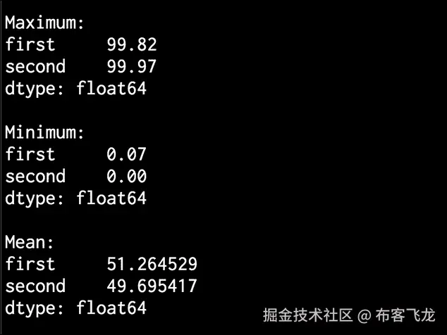
让我们现在开始提取一些统计数据。要提取最大值和最小值,请使用以下代码:
# Print max and min print '\nMaximum:\n', dataframe.max() print '\nMinimum:\n', dataframe.min() -
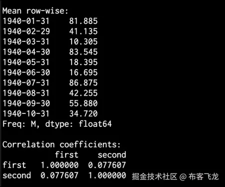
要打印数据的平均值或行平均值,请使用以下代码:
# Print mean print '\nMean:\n', dataframe.mean() print '\nMean row-wise:\n', dataframe.mean(1)[:10] -
滚动平均值是时间序列处理中经常使用的一个重要统计量。最著名的应用之一是平滑信号以消除噪声。滚动平均值是指计算在时间尺度上不断滑动的窗口中信号的平均值。让我们考虑
24的窗口大小,并绘制如下图:# Plot rolling mean pd.rolling_mean(dataframe, window=24).plot() -
相关系数有助于理解数据的性质,如下所示:
# Print correlation coefficients print '\nCorrelation coefficients:\n', dataframe.corr() -
让我们用
60:# Plot rolling correlation plt.figure() pd.rolling_corr(dataframe['first'], dataframe['second'], window=60).plot() plt.show()的窗口大小来绘制这个图
-
The full code is given in the
extract_stats.pyfile that is already provided to you. If you run the code, the rolling mean will look like the following:

- The second output figure indicates the rolling correlation:

- In the upper half of the Terminal, you will see max, min, and mean values printed, as shown in the following image:
- In the lower half of the Terminal, you will see the row-wise mean stats and correlation coefficients printed, as seen in the following image:
建立序列数据的隐马尔可夫模型
当涉及到顺序数据分析时,隐马尔可夫模型 ( HMMs )真的很强大。它们被广泛用于金融、语音分析、天气预报、单词排序等等。我们通常对揭示随时间出现的隐藏模式感兴趣。
任何产生一系列输出的数据源都可能产生模式。请注意,hmm 是生成模型,这意味着一旦他们了解了底层结构,他们就可以生成数据。hmm 不能区分基本形式的类。这与区分模型形成对比,区分模型可以学习区分类,但不能生成数据。
做好准备
例如,假设我们想预测明天天气是晴朗、寒冷还是下雨。为此,我们查看所有参数,如温度、压力等,而底层状态是隐藏的。这里,基础状态指的是三个可用的选项:晴天、冷天或雨天。如果你想了解更多关于头盔显示器的知识,请点击www.robots.ox.ac.uk/~vgg/rg/sli…查看本教程。
我们将使用hmmlearn来构建和培训 hmm。在继续之前,请确保安装了此软件。您可以在hmmlearn.readthedocs.org/en/latest找到安装说明。
怎么做…
-
新建一个 Python 文件,导入以下包:
import datetime import numpy as np import matplotlib.pyplot as plt from hmmlearn.hmm import GaussianHMM from convert_to_timeseries import convert_data_to_timeseries -
我们将使用已经提供给您的名为
data_hmm.txt的文件中的数据。该文件包含逗号分隔的行。每行包含三个值:一年、一个月和一个浮点数据。让我们将它加载到一个 NumPy 数组中:# Load data from input file input_file = 'data_hmm.txt' data = np.loadtxt(input_file, delimiter=',') -
让我们按列堆叠数据进行分析。我们不需要在技术上对它进行列堆叠,因为它只有一列。但是,如果您有多个列要分析,您可以使用以下结构:
# Arrange data for training X = np.column_stack([data[:,2]]) -
使用四个组件创建和训练隐马尔可夫模型。成分的数量是我们必须选择的超参数。这里,通过选择四个,我们说数据是使用四个底层状态生成的。我们将很快看到性能如何随此参数变化:
# Create and train Gaussian HMM print "\nTraining HMM...." num_components = 4 model = GaussianHMM(n_components=num_components, covariance_type="diag", n_iter=1000) model.fit(X) -
运行预测器获取隐藏状态:
# Predict the hidden states of HMM hidden_states = model.predict(X) -
计算隐藏状态的均值和方差:
print "\nMeans and variances of hidden states:" for i in range(model.n_components): print "\nHidden state", i+1 print "Mean =", round(model.means_[i][0], 3) print "Variance =", round(np.diag(model.covars_[i])[0], 3) -
正如我们之前讨论的,hmm 是生成模型。因此,让我们生成例如
1000样本并绘制如下:# Generate data using model num_samples = 1000 samples, _ = model.sample(num_samples) plt.plot(np.arange(num_samples), samples[:,0], c='black') plt.title('Number of components = ' + str(num_components)) plt.show() -
The full code is given in the
hmm.pyfile that is already provided to you. If you run the code, you will see the following figure: -
You can experiment with the
n_componentsparameter to see how the curve gets nicer as you increase it. You can basically give it more freedom to train and customize by allowing a larger number of hidden states. If you increase it to8, you will see the following figure: -
If you increase this to
12, it will get even smoother:

- In the Terminal, you will get the following output:

为连续文本数据构建条件随机字段
条件随机场 ( CRFs )是用于分析结构化数据的概率模型。它们经常用于标记和分割序列数据。通用报告格式是区别模型,而 hmm 是生成模型。通用报告格式被广泛用于分析序列、股票、语音、单词等。在这些模型中,给定一个特定的标记观察序列,我们定义了这个序列的条件概率分布。这与 hmm 形成对比,在 hmm 中,我们定义了标签和观察序列的联合分布。
做好准备
hmm 假设当前输出在统计上独立于以前的输出。这是 hmm 需要的,以确保推理以健壮的方式工作。然而,这个假设不一定总是正确的!时间序列设置中的当前输出通常取决于先前的输出。相对于 hmm,CRF 的主要优势之一是它们本质上是有条件的,这意味着我们不假设输出观测之间有任何独立性。使用通用报告格式比使用 hmm 还有其他一些优势。在许多应用中,如语言学、生物信息学、语音分析等,通用报告格式往往优于 hmm。在这个食谱中,我们将学习如何使用 CRFs 来分析字母序列。
我们将使用名为pystruct的库来构建和训练 CRF。在继续之前,请确保安装了此软件。您可以在pystruct.github.io/installatio…找到安装说明。
怎么做…
-
新建一个 Python 文件,导入以下包:
import os import argparse import cPickle as pickle import numpy as np import matplotlib.pyplot as plt from pystruct.datasets import load_letters from pystruct.models import ChainCRF from pystruct.learners import FrankWolfeSSVM -
定义一个参数解析器,将
C值作为输入参数。C是一个超参数,它控制你希望你的模型有多具体,同时又不会失去归纳的能力:def build_arg_parser(): parser = argparse.ArgumentParser(description='Trains the CRF classifier') parser.add_argument("--c-value", dest="c_value", required=False, type=float, default=1.0, help="The C value that will be used for training") return parser -
定义一个类来处理所有与 CRF 相关的处理:
class CRFTrainer(object): -
定义一个
init函数来初始化值:def __init__(self, c_value, classifier_name='ChainCRF'): self.c_value = c_value self.classifier_name = classifier_name -
我们将使用链式 CRF 来分析数据。我们需要为此添加一个错误检查,如下所示:
if self.classifier_name == 'ChainCRF': model = ChainCRF() -
定义我们将在通用报告格式模型中使用的分类器。我们将使用一种类型的支持向量麻吉 ne 来实现这一点:
self.clf = FrankWolfeSSVM(model=model, C=self.c_value, max_iter=50) else: raise TypeError('Invalid classifier type') -
加载字母数据集。该数据集由分段字母及其相关特征向量组成。我们不会分析图像,因为我们已经有了特征向量。每个单词的第一个字母都被去掉了,所以我们只有小写字母:
def load_data(self): letters = load_letters() -
将数据和标签加载到各自的变量中:
X, y, folds = letters['data'], letters['labels'], letters['folds'] X, y = np.array(X), np.array(y) return X, y, folds -
定义一种训练方法,如下所示:
# X is a numpy array of samples where each sample # has the shape (n_letters, n_features) def train(self, X_train, y_train): self.clf.fit(X_train, y_train) -
定义评估模型性能的方法:
```py
    def evaluate(self, X_test, y_test):
        return self.clf.score(X_test, y_test)
```
11. 定义新数据的分类方法:
```py
    # Run the classifier on input data
    def classify(self, input_data):
        return self.clf.predict(input_data)[0]
```
12. 这些字母被编入一个编号数组。为了检查输出并使其可读,我们需要将这些数字转换成字母。为此定义一个函数:
```py
def decoder(arr):
```

```py
    alphabets = 'abcdefghijklmnopqrstuvwxyz'
    output = ''
    for i in arr:
        output += alphabets[i]

    return output
```
13. 定义函数并解析输入参数:
```py
if __name__=='__main__':
    args = build_arg_parser().parse_args()
    c_value = args.c_value
```
14. 用类和C值初始化变量:
```py
    crf = CRFTrainer(c_value)
```
15. 加载字母数据:
```py
    X, y, folds = crf.load_data()
```
16. 将数据分成训练和测试数据集:
```py
    X_train, X_test = X[folds == 1], X[folds != 1]
    y_train, y_test = y[folds == 1], y[folds != 1]
```
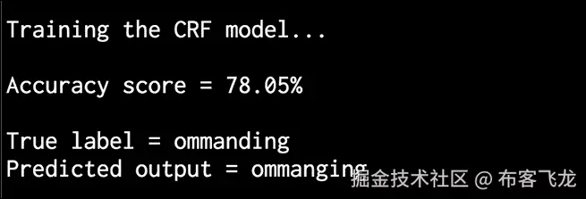
17. 训练通用报告格式模型,如下所示:
```py
    print "\nTraining the CRF model..."
    crf.train(X_train, y_train)
```
18. 评估通用报告格式模型的性能:
```py
    score = crf.evaluate(X_test, y_test)
    print "\nAccuracy score =", str(round(score*100, 2)) + '%'
```
19. 让我们取一个随机测试向量,并使用模型预测输出:
```py
    print "\nTrue label =", decoder(y_test[0])
    predicted_output = crf.classify([X_test[0]])
    print "Predicted output =", decoder(predicted_output)
```
20. The full code is given in the crf.py file that is already provided to you. If you run this code, you will get the following output on your Terminal. As we can see, the word is supposed to be "commanding". The CRF does a pretty good job of predicting all the letters:
利用隐马尔可夫模型分析股市数据
让我们使用隐马尔可夫模型分析股市数据。股市数据是时间序列数据的一个很好的例子,其中数据以日期的形式组织。在我们将要使用的数据集中,我们可以看到不同公司的股票价值是如何随着时间波动的。隐马尔可夫模型是用于分析这种时间序列数据的生成模型。在这个食谱中,我们将使用这些模型来分析股票价值。
怎么做…
-
新建一个 Python 文件,导入以下包:
import datetime import numpy as np import matplotlib.pyplot as plt from matplotlib.finance import quotes_historical_yahoo_ochl from hmmlearn.hmm import GaussianHMM -
从雅虎财经获取股票报价。
matplotlib中有一种方法可以直接加载:# Get quotes from Yahoo finance quotes = quotes_historical_yahoo_ochl("INTC", datetime.date(1994, 4, 5), datetime.date(2015, 7, 3)) -
每个报价中有六个值。让我们提取相关数据,如股票的收盘价和交易的股票数量,以及它们对应的日期:
# Extract the required values dates = np.array([quote[0] for quote in quotes], dtype=np.int) closing_values = np.array([quote[2] for quote in quotes]) volume_of_shares = np.array([quote[5] for quote in quotes])[1:] -
让我们计算每种类型数据的收盘价的百分比变化。我们将使用这作为特征之一:
# Take diff of closing values and computing rate of change diff_percentage = 100.0 * np.diff(closing_values) / closing_values[:-1] dates = dates[1:] -
按列堆叠两个数组进行训练:
# Stack the percentage diff and volume values column-wise for training X = np.column_stack([diff_percentage, volume_of_shares]) -
使用五个组件训练隐马尔可夫模型:
# Create and train Gaussian HMM print "\nTraining HMM...." model = GaussianHMM(n_components=5, covariance_type="diag", n_iter=1000) model.fit(X) -
使用训练好的隐马尔可夫模型生成
500样本并绘制出来,如下所示:# Generate data using model num_samples = 500 samples, _ = model.sample(num_samples) plt.plot(np.arange(num_samples), samples[:,0], c='black') plt.show() -
The full code is given in
hmm_stock.pythat is already provided to you. If you run this code, you will see the following figure:
九、图像内容分析
在本章中,我们将介绍以下食谱:
- 使用 OpenCV-Python 对图像进行操作
- 检测边缘
- 直方图均衡
- 检测拐角
- 检测 SIFT 特征点
- 建筑之星特征探测器
- 使用视觉码本和矢量量化创建特征
- 使用极随机森林训练图像分类器
- 构建对象识别器
简介
计算机视觉是一个研究如何处理、分析和理解视觉数据内容的领域。在图像内容分析中,我们使用大量的计算机视觉算法来建立我们对图像中对象的理解。计算机视觉涵盖了图像分析的各个方面,如目标识别、形状分析、姿态估计、三维建模、视觉搜索等。人类真的很擅长识别和认识周围的事物!计算机视觉的最终目标是利用计算机对人类视觉系统进行精确建模。
计算机视觉由不同层次的分析组成。在低级视觉中,我们处理像素处理任务,例如边缘检测、形态处理和光流。在中级和高级视觉中,我们处理事物,例如对象识别、3D 建模、运动分析以及视觉数据的各种其他方面。随着我们越走越高,我们倾向于更深入地研究我们视觉系统的概念方面,并试图基于活动和意图提取视觉数据的描述。需要注意的一点是,较高层往往依赖较低层的输出进行分析。
这里最常见的一个问题是,“计算机视觉和图像处理有什么不同?”图像处理研究像素级的图像变换。图像处理系统的输入和输出都是图像。一些常见的例子是边缘检测、直方图均衡化或图像压缩。计算机视觉算法在很大程度上依赖图像处理算法来履行其职责。在计算机视觉中,我们处理更复杂的事情,包括在概念层面理解视觉数据。这样做的原因是因为我们想要对图像中的对象进行有意义的描述。计算机视觉系统的输出是给定图像中三维场景的解释。这种解释可以有多种形式,取决于手头的任务。
在本章中,我们将使用一个名为**【OpenCV】**的库来分析图像。OpenCV 是世界上最受欢迎的计算机视觉库。由于它已经针对许多不同的平台进行了高度优化,它已经成为行业中事实上的标准。在继续之前,请确保安装了支持 Python 的库。您可以在opencv.org下载安装 OpenCV。有关各种操作系统的详细安装说明,您可以参考网站上的文档部分。
使用 OpenCV-Python 对图像进行操作
让我们来看看如何使用 OpenCV-Python 对图像进行操作。在这个食谱中,我们将看到如何加载和显示图像。我们还将了解如何裁剪、调整大小以及将图像保存到输出文件中。
怎么做…
-
新建一个 Python 文件,导入以下包:
import sys import cv2 import numpy as np -
将输入图像指定为文件的第一个参数,并使用图像读取函数读取它。我们将使用
forest.jpg,如下所示:# Load and display an image -- 'forest.jpg' input_file = sys.argv[1] img = cv2.imread(input_file) -
显示输入图像,如下所示:
cv2.imshow('Original', img) -
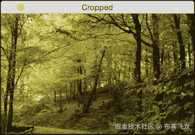
我们现在将裁剪这张图片。提取输入图像的高度和宽度,然后指定边界:
# Cropping an image h, w = img.shape[:2] start_row, end_row = int(0.21*h), int(0.73*h) start_col, end_col= int(0.37*w), int(0.92*w) -
使用 NumPy 样式切片裁剪图像并显示:
img_cropped = img[start_row:end_row, start_col:end_col] cv2.imshow('Cropped', img_cropped) -
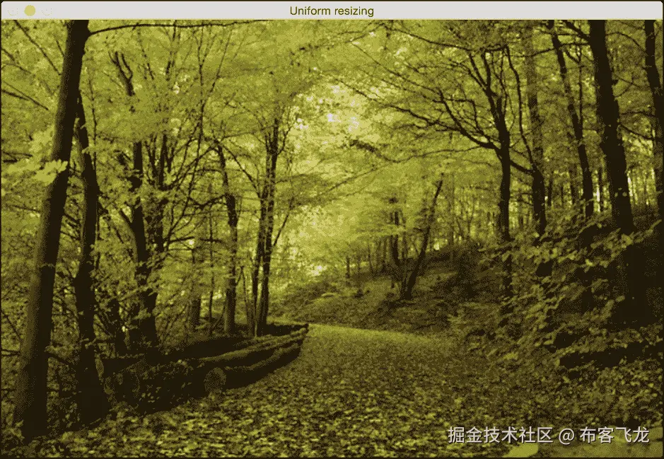
将图像调整到原始尺寸的
1.3倍并显示:# Resizing an image scaling_factor = 1.3 img_scaled = cv2.resize(img, None, fx=scaling_factor, fy=scaling_factor, interpolation=cv2.INTER_LINEAR) cv2.imshow('Uniform resizing', img_scaled) -
前面的方法将在两个维度上统一缩放图像。让我们假设我们想要基于特定的输出维度来扭曲图像。我们使用以下代码:
img_scaled = cv2.resize(img, (250, 400), interpolation=cv2.INTER_AREA) cv2.imshow('Skewed resizing', img_scaled) -
将图像保存到输出文件中:
# Save an image output_file = input_file[:-4] + '_cropped.jpg' cv2.imwrite(output_file, img_cropped) cv2.waitKey() -
waitKey()功能显示图像,直到你按下键盘上的一个键。 -
The full code is given in the
operating_on_images.pyfile that is already provided to you. If you run the code, you will see the following input image:

- The second output is the cropped image:
- The third output is the uniformly resized image:
- The fourth output is the skewed image:

检测边缘
边缘检测是计算机视觉中最流行的技术之一。它在许多应用中用作预处理步骤。让我们看看如何使用不同的边缘检测器来检测输入图像中的边缘。
怎么做…
-
新建一个 Python 文件,导入以下包:
import sys import cv2 import numpy as np -
加载输入图像。我们将使用
chair.jpg:# Load the input image -- 'chair.jpg' # Convert it to grayscale input_file = sys.argv[1] img = cv2.imread(input_file, cv2.IMREAD_GRAYSCALE) -
提取图像的高度和宽度:
h, w = img.shape -
索贝尔滤波器是一种类型的边缘检测器,使用 3x3 内核分别检测水平和垂直边缘。你可以在www.tutorialspoint.com/dip/sobel_o…了解更多。让我们从水平探测器开始:
sobel_horizontal = cv2.Sobel(img, cv2.CV_64F, 1, 0, ksize=5) -
运行垂直索贝尔检测器:
sobel_vertical = cv2.Sobel(img, cv2.CV_64F, 0, 1, ksize=5) -
拉普拉斯边缘检测器在两个方向上检测边缘。你可以在homepages.inf.ed.ac.uk/rbf/HIPR2/l…了解更多。我们使用如下:
laplacian = cv2.Laplacian(img, cv2.CV_64F) -
即使拉普拉斯解决了 Sobel 的缺点,输出仍然非常嘈杂。 Canny 边缘检测器比都强,因为它处理问题的方式。这是一个多阶段的过程,它使用滞后来产生干净的边缘。你可以在homepages.inf.ed.ac.uk/rbf/HIPR2/c…:
canny = cv2.Canny(img, 50, 240)了解更多
-
显示所有输出图像:
cv2.imshow('Original', img) cv2.imshow('Sobel horizontal', sobel_horizontal) cv2.imshow('Sobel vertical', sobel_vertical) cv2.imshow('Laplacian', laplacian) cv2.imshow('Canny', canny) cv2.waitKey() -
The full code is given in the
edge_detector.pyfile that is already provided to you. The original input image looks like the following: -
Here is the horizontal Sobel edge detector output. Note how the detected lines tend to be vertical. This is due the fact that it's a horizontal edge detector, and it tends to detect changes in this direction:

- The vertical Sobel edge detector output looks like the following image:

- Here is the Laplacian edge detector output:

- Canny edge detector detects all the edges nicely, as shown in the following image:

直方图均衡化
直方图均衡化是修改图像像素强度以增强对比度的过程。人眼喜欢对比!这就是为什么几乎所有的相机系统都使用直方图均衡化来使图像看起来好看。有趣的是,直方图均衡化过程对于灰度和彩色图像是不同的。在处理彩色图像时有一个陷阱,我们将在这个食谱中看到它。让我们看看怎么做。
怎么做…
-
新建一个 Python 文件,导入以下包:
import sys import cv2 import numpy as np -
加载输入图像。我们将使用图像,
sunrise.jpg:# Load input image -- 'sunrise.jpg' input_file = sys.argv[1] img = cv2.imread(input_file) -
将图像转换为灰度并显示:
# Convert it to grayscale img_gray = cv2.cvtColor(img, cv2.COLOR_BGR2GRAY) cv2.imshow('Input grayscale image', img_gray) -
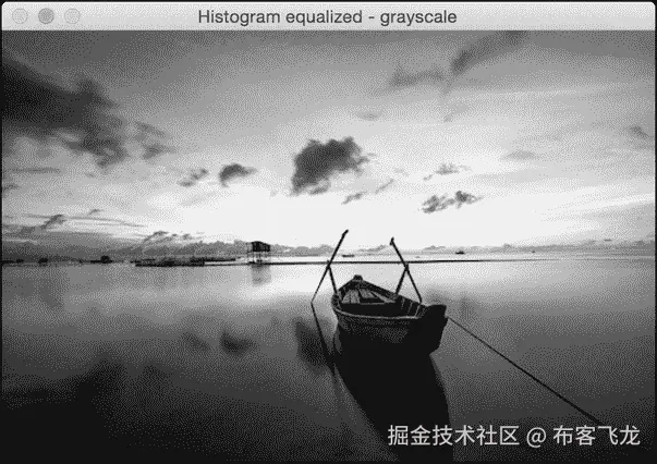
均衡灰度图像的直方图并显示:
# Equalize the histogram img_gray_histeq = cv2.equalizeHist(img_gray) cv2.imshow('Histogram equalized - grayscale', img_gray_histeq) -
为了均衡彩色图像的直方图,我们需要遵循不同的程序。直方图均衡仅适用于强度通道。一幅 RGB 图像由三个颜色通道组成,我们不能对这些通道分别应用直方图均衡化过程。在我们做任何事情之前,我们需要把强度信息和颜色信息分开。所以,我们先把它转换成 YUV 色彩空间,均衡 Y 通道,然后再转换回 RGB 得到输出。您可以在softpixel.com/~cwright/pr…了解更多关于 YUV 色彩空间的信息。OpenCV 默认加载 BGR 格式的图像,所以我们先把它从 BGR 转换成 YUV:
# Histogram equalization of color images img_yuv = cv2.cvtColor(img, cv2.COLOR_BGR2YUV) -
均衡 Y 通道,如下所示:
img_yuv[:,:,0] = cv2.equalizeHist(img_yuv[:,:,0]) -
将其转换回 BGR:
img_histeq = cv2.cvtColor(img_yuv, cv2.COLOR_YUV2BGR) -
显示输入和输出图像:
cv2.imshow('Input color image', img) cv2.imshow('Histogram equalized - color', img_histeq) cv2.waitKey() -
The full code is given in the
histogram_equalizer.pyfile that is already provided to you. The input image is shown, as follows: -
The histogram equalized image looks like the following:
检测拐角
角点检测是计算机视觉中的一个重要过程。它帮助我们识别图像中的显著点。这是最早用于开发图像分析系统的特征提取技术之一。
怎么做…
-
新建一个 Python 文件,导入以下包:
import sys import cv2 import numpy as np -
加载输入图像。我们将使用
box.png:# Load input image -- 'box.png' input_file = sys.argv[1] img = cv2.imread(input_file) cv2.imshow('Input image', img) -
将图像转换为灰度并将其转换为浮点值。我们需要角点检测器的浮点值来工作:
img_gray = cv2.cvtColor(img, cv2.COLOR_BGR2GRAY) img_gray = np.float32(img_gray) -
在灰度图像上运行 哈里斯角点检测器功能。您可以在了解更多关于哈里斯角点检测器的信息
-
为了标记拐角,我们需要放大图像,如下所示:
# Resultant image is dilated to mark the corners img_harris = cv2.dilate(img_harris, None) -
让我们对图像进行阈值化,以显示重要的点:
# Threshold the image img[img_harris > 0.01 * img_harris.max()] = [0, 0, 0] -
显示输出图像:
cv2.imshow('Harris Corners', img) cv2.waitKey() -
The full code is given in the
corner_detector.pyfile that is already provided to you. The input image is displayed, as follows: -
The output image after detecting corners is as follows:
检测 SIFT 特征点
尺度不变特征变换 ( SIFT )是计算机视觉领域最受欢迎的特征之一。大卫·劳在他的开创性论文中首次提出了这一点,该论文可在 www.cs.ubc.ca/~lowe/paper… 获得。从那时起,它已经成为用于图像识别和内容分析的最有效的功能之一。它对规模、方向、强度等具有鲁棒性。这构成了我们物体识别系统的基础。让我们来看看如何检测这些特征点。
怎么做…
-
新建一个 Python 文件,导入以下包:
import sys import cv2 import numpy as np -
加载输入图像。我们将使用
table.jpg:# Load input image -- 'table.jpg' input_file = sys.argv[1] img = cv2.imread(input_file) -
将此图像转换为灰度:
img_gray = cv2.cvtColor(img, cv2.COLOR_BGR2GRAY) -
初始化 SIFT 检测器对象并提取关键点:
sift = cv2.xfeatures2d.SIFT_create() keypoints = sift.detect(img_gray, None) -
关键点是显著点,但不是特征。这基本上给了我们突出点的位置。SIFT 也是一个非常有效的特征提取器,但是我们将在后面的食谱中看到它的这一方面。
-
在输入图像的顶部绘制关键点,如下所示:
img_sift = np.copy(img) cv2.drawKeypoints(img, keypoints, img_sift, flags=cv2.DRAW_MATCHES_FLAGS_DRAW_RICH_KEYPOINTS) -
显示输入和输出图像:
cv2.imshow('Input image', img) cv2.imshow('SIFT features', img_sift) cv2.waitKey() -
The full code is given in the
feature_detector.pyfile that is already provided to you. The input image is as follows: -
The output image looks like the following:
构建星特征检测器
SIFT 特征检测器在很多情况下都不错。然而,当我们构建对象识别系统时,我们可能希望在使用 SIFT 提取特征之前使用不同的特征检测器。这将使我们能够灵活地级联不同的块,以获得最佳性能。所以,在这种情况下,我们将使用恒星特征检测器来看看如何做到这一点。
怎么做…
-
新建一个 Python 文件,导入以下包:
import sys import cv2 import numpy as np -
定义一个类来处理所有与星特征检测相关的功能:
class StarFeatureDetector(object): def __init__(self): self.detector = cv2.xfeatures2d.StarDetector_create() -
定义在输入图像上运行检测器的功能:
def detect(self, img): return self.detector.detect(img) -
在
main功能中加载输入图像。我们将使用table.jpg:T2 -
将图像转换为灰度:
# Convert to grayscale img_gray = cv2.cvtColor(input_img, cv2.COLOR_BGR2GRAY) -
使用星形特征检测器检测特征:
# Detect features using Star feature detector keypoints = StarFeatureDetector().detect(input_img) -
在输入图像上绘制关键点:
cv2.drawKeypoints(input_img, keypoints, input_img, flags=cv2.DRAW_MATCHES_FLAGS_DRAW_RICH_KEYPOINTS) -
显示输出图像:
cv2.imshow('Star features', input_img) cv2.waitKey() -
The full code is given in the
star_detector.pyfile that is already provided to you. The output image looks like the following:
使用视觉码本和矢量量化创建特征
为了构建一个物体识别系统,我们需要从每个图像中提取特征向量。每个图像需要有一个签名,可以用于匹配。我们使用一个名为 的概念来构建图像签名。该码本基本上是字典,我们将使用它来为训练数据集中的图像提供表示。我们使用矢量量化来聚类许多特征点,并得出质心。这些质心将作为我们视觉码本的元素。您可以在http://mi . eng . cam . AC . uk/~ cipolla/讲座/PartIb/old/IB-visualcodebook . pdf了解更多信息。
在你开始之前,确保你有一些训练图像。给你提供了一个包含三个类的样本训练数据集,每个类有 20 个图像。这些图片是从www.vision.caltech.edu/html-files/…下载的。
要建立一个健壮的物体识别系统,你需要成千上万的图像。有一个叫做Caltech256的数据集,在这个领域非常流行!它包含 256 类图像,每个类包含数千个样本。您可以在www.vision.caltech.edu/Image_Datas…下载该数据集。
怎么做…
-
这是一个冗长的食谱,所以我们只看重要的功能。完整的代码在已经提供给你的
build_features.py文件中给出。让我们来看看为提取特征而定义的类:class FeatureBuilder(object): -
定义从输入图像中提取特征的方法。我们将使用星检测器获取关键点,然后使用 SIFT 从这些位置提取描述符:
def extract_ features(self, img): keypoints = StarFeatureDetector().detect(img) keypoints, feature_vectors = compute_sift_features(img, keypoints) return feature_vectors -
我们需要从所有描述符中提取质心:
def get_codewords(self, input_map, scaling_size, max_samples=12): keypoints_all = [] count = 0 cur_label = '' -
每个图像将产生大量描述符。我们将只使用少量图像,因为质心在此之后不会有太大变化:
for item in input_map: if count >= max_samples: if cur_class != item['object_class']: count = 0 else: continue count += 1 -
打印进度如下:
if count == max_samples: print "Built centroids for", item['object_class'] -
提取当前标签:
cur_class = item['object_class'] -
读取图像并调整大小:
img = cv2.imread(item['image_path']) img = resize_image(img, scaling_size) -
将维数设置为 128,提取特征:
num_dims = 128 feature_vectors = self.extract_image_features(img) keypoints_all.extend(feature_vectors) -
使用矢量量化对特征点进行量化。矢量量化是N-维版本的“四舍五入”。你可以在www.data-compression.com/vq.shtml了解更多。
kmeans, centroids = BagOfWords().cluster(keypoints_all) return kmeans, centroids -
定义处理词包模型和矢量量化的类:
```py
class BagOfWords(object):
    def __init__(self, num_clusters=32):
        self.num_dims = 128
        self.num_clusters = num_clusters
        self.num_retries = 10
```
11. 定义量化数据点的方法。我们将使用 k-means 聚类来实现这一点:
```py
def cluster(self, datapoints):
    kmeans = KMeans(self.num_clusters,
        n_init=max(self.num_retries, 1),
        max_iter=10, tol=1.0)
```
12. 提取质心,如下所示:
```py
    res = kmeans.fit(datapoints)
    centroids = res.cluster_centers_
    return kmeans, centroids
```
13. 定义一种数据归一化的方法:
```py
def normalize(self, input_data):
    sum_input = np.sum(input_data)

    if sum_input > 0:
        return input_data / sum_input
    else:
        return input_data
```
14. 定义一种获取特征向量的方法:
```py
def construct_feature(self, img, kmeans, centroids):
    keypoints = StarFeatureDetector().detect(img)
    keypoints, feature_vectors = compute_sift_features(img, keypoints)
    labels = kmeans.predict(feature_vectors)
    feature_vector = np.zeros(self.num_clusters)
```
15. 建立直方图并归一化:
```py
    for i, item in enumerate(feature_vectors):
        feature_vector[labels[i]] += 1

        feature_vector_img = np.reshape(feature_vector,
((1, feature_vector.shape[0])))
        return self.normalize(feature_vector_img)
```
16. Define a method the extract the SIFT features:
```py
# Extract SIFT features
def compute_sift_features(img, keypoints):
    if img is None:
        raise TypeError('Invalid input image')

    img_gray = cv2.cvtColor(img, cv2.COLOR_BGR2GRAY)
    keypoints, descriptors = cv2.xfeatures2d.SIFT_create().compute(img_gray, keypoints)
    return keypoints, descriptors
```

如前所述,完整的代码请参考 build_features.py。您应该以下列方式运行代码:

```py
$ python build_features.py –-data-folder /path/to/training_img/ --codebook-file codebook.pkl --feature-map-file feature_map.pkl

```

这将生成两个名为`codebook.pkl`和`feature_map.pkl`的文件。我们将在下一个食谱中使用这些文件。
使用极随机森林训练图像分类器
我们将使用 【极随机森林】 ( ERFs )来训练我们的图像分类器。物体识别系统使用图像分类器将图像分类成已知的类别。由于的速度和精度,ERFs 在机器学习领域非常受欢迎。我们基本上构建了一堆基于我们的图像签名的决策树,然后训练森林做出正确的决定。你可以在https://www . stat . Berkeley . edu/~ brei man/RandomForests/cc _ home . htm了解更多随机森林。您可以在http://www . Monte fiore . ulg . AC . be/~ Ernst/uploads/news/id63/extreme-random-trees . pdf了解 ERFs。
怎么做…
-
新建一个 Python 文件,导入以下包:
import argparse import cPickle as pickle import numpy as np from sklearn.ensemble import ExtraTreesClassifier from sklearn import preprocessing -
定义参数解析器:
def build_arg_parser(): parser = argparse.ArgumentParser(description='Trains the classifier') parser.add_argument("--feature-map-file", dest="feature_map_file", required=True, help="Input pickle file containing the feature map") parser.add_argument("--model-file", dest="model_file", required=False, help="Output file where the trained model will be stored") return parser -
定义一个类来处理电流变流体培训。我们将使用标签编码器来编码我们的训练标签:
class ERFTrainer(object): def __init__(self, X, label_words): self.le = preprocessing.LabelEncoder() self.clf = ExtraTreesClassifier(n_estimators=100, max_depth=16, random_state=0) -
编码标签并训练分类器:
y = self.encode_labels(label_words) self.clf.fit(np.asarray(X), y) -
定义一个函数来编码标签:
def encode_labels(self, label_words): self.le.fit(label_words) return np.array(self.le.transform(label_words), dtype=np.float32) -
定义一个函数对未知数据点进行分类:
def classify(self, X): label_nums = self.clf.predict(np.asarray(X)) label_words = self.le.inverse_transform([int(x) for x in label_nums]) return label_words -
定义
main函数并解析输入参数:if __name__=='__main__': args = build_arg_parser().parse_args() feature_map_file = args.feature_map_file model_file = args.model_file -
加载我们在上一个食谱中创建的特征图:
# Load the feature map with open(feature_map_file, 'r') as f: feature_map = pickle.load(f) -
提取特征向量:
# Extract feature vectors and the labels label_words = [x['object_class'] for x in feature_map] dim_size = feature_map[0]['feature_vector'].shape[1] X = [np.reshape(x['feature_vector'], (dim_size,)) for x in feature_map] -
培训电流变流体,基于培训数据:
```py
    # Train the Extremely Random Forests classifier
    erf = ERFTrainer(X, label_words)
```
11. 保存训练好的电流变液模型,如下所示:
```py
    if args.model_file:
        with open(args.model_file, 'w') as f:
            pickle.dump(erf, f)
```
12. The full code is given in the trainer.py file that is provided to you. You should run the code in the following way:
```py
$ python trainer.py --feature-map-file feature_map.pkl --model-file erf.pkl

```

这将生成一个名为`erf.pkl`的文件。我们将在下一个食谱中使用这个文件。
构建对象识别器
现在我们训练了一个 ERF 模型,让我们继续构建一个可以识别未知图像内容的对象识别器。
怎么做…
-
新建一个 Python 文件,导入以下包:
import argparse import cPickle as pickle import cv2 import numpy as np import build_features as bf from trainer import ERFTrainer -
定义参数解析器:
def build_arg_parser(): parser = argparse.ArgumentParser(description='Extracts features \ from each line and classifies the data') parser.add_argument("--input-image", dest="input_image", required=True, help="Input image to be classified") parser.add_argument("--model-file", dest="model_file", required=True, help="Input file containing the trained model") parser.add_argument("--codebook-file", dest="codebook_file", required=True, help="Input file containing the codebook") return parser -
定义一个类来处理图像标签提取功能:
class ImageTagExtractor(object): def __init__(self, model_file, codebook_file): with open(model_file, 'r') as f: self.erf = pickle.load(f) with open(codebook_file, 'r') as f: self.kmeans, self.centroids = pickle.load(f) -
使用训练好的电流变流体模型定义一个函数来预测输出:
def predict(self, img, scaling_size): img = bf.resize_image(img, scaling_size) feature_vector = bf.BagOfWords().construct_feature( img, self.kmeans, self.centroids) image_tag = self.erf.classify(feature_vector)[0] return image_tag -
定义
main功能,加载输入图像:if __name__=='__main__': args = build_arg_parser().parse_args() model_file = args.model_file codebook_file = args.codebook_file input_image = cv2.imread(args.input_image) -
适当缩放图像,如下所示:
scaling_size = 200 -
在终端上打印输出:
print "\nOutput:", ImageTagExtractor(model_file, codebook_file).predict(input_image, scaling_size) -
The full code is given in the
object_recognizer.pyfile that is already provided to you. You should run the code in the following way:$ python object_recognizer.py --input-image imagefile.jpg --model-file erf.pkl --codebook-file codebook.pkl您将看到终端上打印的输出类。
十、生物识别人脸识别
在本章中,我们将介绍以下食谱:
- 从网络摄像头捕捉和处理视频
- 使用哈尔级联构建人脸检测器
- 构建眼睛和鼻子探测器
- 执行主成分分析
- 执行核心主成分分析
- 执行盲源分离
- 利用局部二值模式直方图构建人脸识别器
简介
人脸识别是指在给定的图像中识别人的任务。这与人脸检测不同,在人脸检测中,我们在给定的图像中定位人脸。在人脸检测过程中,我们不在乎这个人是谁。我们只是识别图像中包含人脸的区域。因此,在典型的生物特征人脸识别系统中,我们需要确定人脸的位置才能识别它。
人脸识别对人类来说非常容易。我们似乎毫不费力地做到了,而且我们一直都在这样做!我们如何让机器做同样的事情?我们需要了解面部的哪些部位可以用来唯一地识别一个人。我们的大脑有一个内部结构,它似乎对特定的特征做出反应,比如边缘、角落、运动等等。人类视觉皮层将所有这些特征结合成一个连贯的推论。如果我们想让我们的机器准确地识别人脸,我们需要用类似的方式来表述这个问题。我们需要从输入图像中提取特征,并将其转换为有意义的表示。
从网络摄像头捕捉和处理视频
我们将在本章中使用网络摄像头来捕获视频数据。让我们看看如何使用 OpenCV-Python 从网络摄像头捕捉视频。
怎么做…
-
新建一个 Python 文件,导入以下包:
import cv2 -
OpenCV 提供了一个视频捕获对象,我们可以使用它从网络摄像头中捕获图像。
0输入参数指定网络摄像头的 ID。如果你连接一个 USB 摄像头,那么它会有一个不同的 ID:# Initialize video capture object cap = cv2.VideoCapture(0) -
定义使用网络摄像头拍摄的帧的比例因子:
# Define the image size scaling factor scaling_factor = 0.5 -
开始一个无限循环,并保持捕捉帧,直到您按下 Esc 键。从网络摄像头读取画面:
# Loop until you hit the Esc key while True: # Capture the current frame ret, frame = cap.read() -
调整框架大小是可选的,但在代码中仍然是有用的:
# Resize the frame frame = cv2.resize(frame, None, fx=scaling_factor, fy=scaling_factor, interpolation=cv2.INTER_AREA) -
显示画面:
# Display the image cv2.imshow('Webcam', frame) -
等待 1 ms,然后捕捉下一帧:
# Detect if the Esc key has been pressed c = cv2.waitKey(1) if c == 27: break -
释放视频拍摄对象:
# Release the video capture object cap.release() -
退出代码前关闭所有活动窗口:
# Close all active windows cv2.destroyAllWindows() -
The full code is given in the
video_capture.pyfile that's already provided to you for reference. If you run this code, you will see the video from the webcam, similar to the following screenshot:

使用哈尔级联构建人脸检测器
正如我们前面讨论的,人脸检测是确定人脸在输入图像中的位置的过程。我们将使用哈尔级联进行人脸检测。这是通过在多个尺度上从图像中提取大量简单特征来实现的。简单的特征基本上是非常容易计算的边、线和矩形特征。然后通过创建一系列简单的分类器来训练它。 自适应增压技术用于使该过程稳健。可以在http://docs . opencv . org/3 . 1 . 0/D7/d8b/tutorial _ py _ face _ detection . html # GSC . tab = 0了解更多。让我们来看看如何在网络摄像头拍摄的视频帧中确定人脸的位置。
怎么做…
-
新建一个 Python 文件,导入以下包:
import cv2 import numpy as np -
加载面探测器级联文件。这是一个训练好的模型,我们可以用作检测器:
# Load the face cascade file face_cascade = cv2.CascadeClassifier('cascade_files/haarcascade_frontalface_alt.xml') -
检查级联文件是否加载正确:
# Check if the face cascade file has been loaded if face_cascade.empty(): raise IOError('Unable to load the face cascade classifier xml file') -
创建视频采集对象:
# Initialize the video capture object cap = cv2.VideoCapture(0) -
定义图像下采样的比例因子:
# Define the scaling factor scaling_factor = 0.5 -
继续循环直到你按下 Esc 键:
# Loop until you hit the Esc key while True: # Capture the current frame and resize it ret, frame = cap.read() -
调整框架大小:
frame = cv2.resize(frame, None, fx=scaling_factor, fy=scaling_factor, interpolation=cv2.INTER_AREA) -
将图像转换为灰度。我们需要灰度图像来运行面部检测器:
# Convert to grayscale gray = cv2.cvtColor(frame, cv2.COLOR_BGR2GRAY) -
对灰度图像运行面部检测器。
1.3参数是指每个阶段的比例乘数。5参数是指每个候选矩形应该具有的最小邻居数量,以便我们可以保留它。这个候选矩形基本上是一个有可能检测到人脸的潜在区域:# Run the face detector on the grayscale image face_rects = face_cascade.detectMultiScale(gray, 1.3, 5) -
对于每个检测到的人脸区域,在它周围画一个矩形:
```py
    # Draw rectangles on the image
    for (x,y,w,h) in face_rects:
        cv2.rectangle(frame, (x,y), (x+w,y+h), (0,255,0), 3)
```
11. 显示输出图像:
```py
    # Display the image
    cv2.imshow('Face Detector', frame)
```
12. 等待 1 ms,然后进行下一次迭代。如果用户按下 Esc 键,跳出循环:
```py
    # Check if Esc key has been pressed
    c = cv2.waitKey(1)
    if c == 27:
        break
```
13. 退出代码前释放并销毁对象:
```py
# Release the video capture object and close all windows
cap.release()
cv2.destroyAllWindows()
```
14. The full code is given in the face_detector.py file that's already provided to you for reference. If you run this code, you will see the face being detected in the webcam video:

建造眼睛和鼻子探测器
哈尔级联方法可以扩展到检测所有类型的物体。让我们看看如何使用它来检测输入视频中的眼睛和鼻子。
怎么做…
-
新建一个 Python 文件,导入以下包:
import cv2 import numpy as np -
加载面部、眼睛和鼻子级联文件:
# Load face, eye, and nose cascade files face_cascade = cv2.CascadeClassifier('cascade_files/haarcascade_frontalface_alt.xml') eye_cascade = cv2.CascadeClassifier('cascade_files/haarcascade_eye.xml') nose_cascade = cv2.CascadeClassifier('cascade_files/haarcascade_mcs_nose.xml') -
检查文件是否正确加载:
# Check if face cascade file has been loaded if face_cascade.empty(): raise IOError('Unable to load the face cascade classifier xml file') # Check if eye cascade file has been loaded if eye_cascade.empty(): raise IOError('Unable to load the eye cascade classifier xml file') # Check if nose cascade file has been loaded if nose_cascade.empty(): raise IOError('Unable to load the nose cascade classifier xml file') -
初始化视频采集对象:
# Initialize video capture object and define scaling factor cap = cv2.VideoCapture(0) -
定义比例因子:
scaling_factor = 0.5 -
继续循环,直到用户按下 Esc 键:
while True: # Read current frame, resize it, and convert it to grayscale ret, frame = cap.read() -
调整框架大小:
frame = cv2.resize(frame, None, fx=scaling_factor, fy=scaling_factor, interpolation=cv2.INTER_AREA) -
将图像转换为灰度:
gray = cv2.cvtColor(frame, cv2.COLOR_BGR2GRAY) -
在灰度图像上运行人脸检测器:
# Run face detector on the grayscale image faces = face_cascade.detectMultiScale(gray, 1.3, 5) -
因为我们知道眼睛和鼻子总是在脸上,所以我们只能在面部区域运行这些检测器:
```py
    # Run eye and nose detectors within each face rectangle
    for (x,y,w,h) in faces:
```
11. 提取人脸感兴趣区域:
```py
        # Grab the current ROI in both color and grayscale images
        roi_gray = gray[y:y+h, x:x+w]
        roi_color = frame[y:y+h, x:x+w]
```
12. 运行眼睛检测器:
```py
        # Run eye detector in the grayscale ROI
        eye_rects = eye_cascade.detectMultiScale(roi_gray)
```
13. 运行鼻子检测器:
```py
        # Run nose detector in the grayscale ROI
        nose_rects = nose_cascade.detectMultiScale(roi_gray, 1.3, 5)
```
14. 在眼睛周围画圈:
```py
        # Draw green circles around the eyes
        for (x_eye, y_eye, w_eye, h_eye) in eye_rects:
            center = (int(x_eye + 0.5*w_eye), int(y_eye + 0.5*h_eye))
            radius = int(0.3 * (w_eye + h_eye))
            color = (0, 255, 0)
            thickness = 3
            cv2.circle(roi_color, center, radius, color, thickness)
```
15. 在鼻子周围画一个矩形:
```py
        for (x_nose, y_nose, w_nose, h_nose) in nose_rects:
            cv2.rectangle(roi_color, (x_nose, y_nose), (x_nose+w_nose,
                y_nose+h_nose), (0,255,0), 3)
            break
```
16. 显示图像:
```py
    # Display the image
    cv2.imshow('Eye and nose detector', frame)
```
17. 等待 1 ms,然后进行下一次迭代。如果用户按下 Esc 键,则断开循环。
```py
    # Check if Esc key has been pressed
    c = cv2.waitKey(1)
    if c == 27:
        break
```
18. 退出代码前释放并销毁对象。
```py
# Release video capture object and close all windows
cap.release()
cv2.destroyAllWindows()
```
19. The full code is given in the eye_nose_detector.py file that's already provided to you for reference. If you run this code, you will see the eyes and nose being detected in the webcam video:

进行主成分分析
主成分分析 ( 主成分分析)是一种降维技术,在计算机视觉和机器学习中使用非常频繁。当我们处理大维度的特征时,训练机器学习系统变得极其昂贵。因此,在训练一个系统之前,我们需要降低数据的维数。然而,当我们降低维度时,我们不想丢失数据中存在的信息。这就是 PCA 进入画面的地方!主成分分析识别数据的重要组成部分,并按重要性顺序排列。你可以在dai.fmph.uniba.sk/courses/ml/…了解更多。它在人脸识别系统中被大量使用。让我们看看如何对输入数据执行 PCA。
怎么做…
-
新建一个 Python 文件,导入以下包:
import numpy as np from sklearn import decomposition -
让我们为输入数据定义五个维度。前两个维度将是独立的,但后三个维度将依赖于前两个维度。这基本上意味着我们可以在没有最后三个维度的情况下生活,因为它们没有给我们任何新的信息:
# Define individual features x1 = np.random.normal(size=250) x2 = np.random.normal(size=250) x3 = 2*x1 + 3*x2 x4 = 4*x1 - x2 x5 = x3 + 2*x4 -
让我们用这些特征创建一个数据集。
# Create dataset with the above features X = np.c_[x1, x3, x2, x5, x4] -
创建主成分分析对象:
# Perform Principal Components Analysis pca = decomposition.PCA() -
在输入数据上拟合主成分分析模型:
pca.fit(X) -
打印尺寸差异:
# Print variances variances = pca.explained_variance_ print '\nVariances in decreasing order:\n', variances -
如果某个特定的维度是有用的,那么它将具有有意义的方差值。让我们设定一个阈值,并确定重要的维度:
# Find the number of useful dimensions thresh_variance = 0.8 num_useful_dims = len(np.where(variances > thresh_variance)[0]) print '\nNumber of useful dimensions:', num_useful_dims -
就像我们之前讨论的,主成分分析发现在这个数据集中只有两个维度是重要的:
# As we can see, only the 2 first components are useful pca.n_components = num_useful_dims -
让我们将数据集从五维集转换为二维集:
X_new = pca.fit_transform(X) print '\nShape before:', X.shape print 'Shape after:', X_new.shape -
The full code is given in the
pca.pyfile that's already provided to you for reference. If you run this code, you will see the following on your Terminal:

进行核主成分分析
主成分分析擅长减少维数,但它以线性方式工作。如果数据不是以线性方式组织的,主成分分析就不能完成要求的工作。这就是内核主成分分析进入画面的地方。你可以在上了解更多。让我们看看如何对输入数据执行内核主成分分析,并将其与主成分分析对相同数据的执行进行比较。
怎么做…
-
新建一个 Python 文件,导入以下包:
import numpy as np import matplotlib.pyplot as plt from sklearn.decomposition import PCA, KernelPCA from sklearn.datasets import make_circles -
定义随机数生成器的种子值。这是生成数据样本进行分析所需要的:
# Set the seed for random number generator np.random.seed(7) -
生成同心圆分布的数据,以演示在这种情况下 PCA 如何不起作用:
# Generate samples X, y = make_circles(n_samples=500, factor=0.2, noise=0.04) -
对该数据进行主成分分析:
# Perform PCA pca = PCA() X_pca = pca.fit_transform(X) -
对该数据进行核主成分分析:
# Perform Kernel PCA kernel_pca = KernelPCA(kernel="rbf", fit_inverse_transform=True, gamma=10) X_kernel_pca = kernel_pca.fit_transform(X) X_inverse = kernel_pca.inverse_transform(X_kernel_pca) -
绘制原始输入数据:
# Plot original data class_0 = np.where(y == 0) class_1 = np.where(y == 1) plt.figure() plt.title("Original data") plt.plot(X[class_0, 0], X[class_0, 1], "ko", mfc='none') plt.plot(X[class_1, 0], X[class_1, 1], "kx") plt.xlabel("1st dimension") plt.ylabel("2nd dimension") -
绘制主成分分析转换数据:
# Plot PCA projection of the data plt.figure() plt.plot(X_pca[class_0, 0], X_pca[class_0, 1], "ko", mfc='none') plt.plot(X_pca[class_1, 0], X_pca[class_1, 1], "kx") plt.title("Data transformed using PCA") plt.xlabel("1st principal component") plt.ylabel("2nd principal component") -
绘制内核主成分分析转换数据:
# Plot Kernel PCA projection of the data plt.figure() plt.plot(X_kernel_pca[class_0, 0], X_kernel_pca[class_0, 1], "ko", mfc='none') plt.plot(X_kernel_pca[class_1, 0], X_kernel_pca[class_1, 1], "kx") plt.title("Data transformed using Kernel PCA") plt.xlabel("1st principal component") plt.ylabel("2nd principal component") -
使用 Kernel 方法将数据转换回原始空间,以显示保留了逆空间:
# Transform the data back to original space plt.figure() plt.plot(X_inverse[class_0, 0], X_inverse[class_0, 1], "ko", mfc='none') plt.plot(X_inverse[class_1, 0], X_inverse[class_1, 1], "kx") plt.title("Inverse transform") plt.xlabel("1st dimension") plt.ylabel("2nd dimension") plt.show() -
The full code is given in the
kpca.pyfile that's already provided to you for reference. If you run this code, you will see four figures. The first figure is the original data:

第二个图描述了使用主成分分析转换的数据:

第三幅图描绘了使用核主成分分析转换的数据。请注意图中右侧的点是如何聚集的:

第四张图描绘了数据到原始空间的逆变换:

执行盲源分离
盲源分离指的是从混合物中分离信号的过程。假设一堆不同的信号发生器产生信号,一个公共接收器接收所有这些信号。现在,我们的工作是利用这些信号的特性从混合物中分离出这些信号。我们将使用 独立分量分析 ( ICA )来实现这一点。你可以在http://www . MIT . edu/~ gari/teaching/6.555/LEASE _ NOtes/ch15 _ BSS . pdf了解更多。让我们看看怎么做。
怎么做…
-
新建一个 Python 文件,导入以下包:
import numpy as np import matplotlib.pyplot as plt from scipy import signal from sklearn.decomposition import PCA, FastICA -
我们将使用已经提供给您的
mixture_of_signals.txt文件中的数据。让我们加载数据:# Load data input_file = 'mixture_of_signals.txt' X = np.loadtxt(input_file) -
创建独立分量分析对象:
# Compute ICA ica = FastICA(n_components=4) -
基于独立分量分析重构信号:
# Reconstruct the signals signals_ica = ica.fit_transform(X) -
提取混合矩阵:
# Get estimated mixing matrix mixing_mat = ica.mixing_ -
进行主成分分析比较:
# Perform PCA pca = PCA(n_components=4) signals_pca = pca.fit_transform(X) # Reconstruct signals based on orthogonal components -
定义要绘制的信号列表:
# Specify parameters for output plots models = [X, signals_ica, signals_pca] -
指定图的颜色:
colors = ['blue', 'red', 'black', 'green'] -
绘制输入信号:
# Plotting input signal plt.figure() plt.title('Input signal (mixture)') for i, (sig, color) in enumerate(zip(X.T, colors), 1): plt.plot(sig, color=color) -
绘制独立分量分析分离信号:
```py
# Plotting ICA signals
plt.figure()
plt.title('ICA separated signals')
plt.subplots_adjust(left=0.1, bottom=0.05, right=0.94,
        top=0.94, wspace=0.25, hspace=0.45)
```
11. 用不同的颜色绘制支线剧情:
```py
for i, (sig, color) in enumerate(zip(signals_ica.T, colors), 1):
    plt.subplot(4, 1, i)
    plt.title('Signal ' + str(i))
    plt.plot(sig, color=color)
```
12. 绘制主成分分析分离信号:
```py
# Plotting PCA signals
plt.figure()
plt.title('PCA separated signals')
plt.subplots_adjust(left=0.1, bottom=0.05, right=0.94,
        top=0.94, wspace=0.25, hspace=0.45)
```
13. 在每个子剧情中使用不同的颜色:
```py
for i, (sig, color) in enumerate(zip(signals_pca.T, colors), 1):
    plt.subplot(4, 1, i)
    plt.title('Signal ' + str(i))
    plt.plot(sig, color=color)

plt.show()
```
14. The full code is given in the blind_source_separation.py file that's already provided to you for reference. If you run this code, you will see three figures. The first figure depicts the input, which is a mixture of signals:

第二幅图描绘了使用独立分量分析分离的信号:
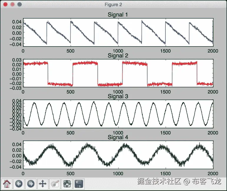
第三幅图描绘了使用主成分分析分离的信号:

利用局部二值模式直方图构建人脸识别器
我们现在准备构建一个人脸识别器。我们需要一个人脸数据集进行训练,所以我们给你提供了一个名为faces_dataset的文件夹,里面包含了少量足以进行训练的图像。该数据集是可在上获得的数据集的子集。这个数据集包含了大量的图像,我们可以用来训练一个人脸识别系统。
我们将使用局部二值模式直方图来构建我们的人脸识别系统。在我们的数据集中,你会看到不同的人。我们的工作是建立一个系统,可以学会将这些人彼此分开。当我们看到一个未知的图像时,这个系统会把它分配给一个现有的类。您可以在上了解更多关于本地二进制模式直方图的信息。来看看如何构建人脸识别器。
怎么做…
-
新建一个 Python 文件,导入以下包:
import os import cv2 import numpy as np from sklearn import preprocessing -
让我们定义一个类来处理与类的标签编码相关的所有任务:
# Class to handle tasks related to label encoding class LabelEncoder(object): -
定义一种对标签进行编码的方法。在输入的训练数据中,标签由单词表示。然而,我们需要数字来训练我们的系统。该方法将定义一个预处理器对象,该对象可以通过维护向前和向后映射来以有组织的方式将单词转换为数字:
# Method to encode labels from words to numbers def encode_labels(self, label_words): self.le = preprocessing.LabelEncoder() self.le.fit(label_words) -
定义一种将单词转换成数字的方法:
# Convert input label from word to number def word_to_num(self, label_word): return int(self.le.transform([label_word])[0]) -
定义一种将数字转换回原始单词的方法:
# Convert input label from number to word def num_to_word(self, label_num): return self.le.inverse_transform([label_num])[0] -
定义从输入文件夹中提取图像和标签的方法:
# Extract images and labels from input path def get_images_and_labels(input_path): label_words = [] -
递归迭代输入文件夹,提取所有图像路径:
# Iterate through the input path and append files for root, dirs, files in os.walk(input_path): for filename in (x for x in files if x.endswith('.jpg')): filepath = os.path.join(root, filename) label_words.append(filepath.split('/')[-2]) -
初始化变量:
# Initialize variables images = [] le = LabelEncoder() le.encode_labels(label_words) labels = [] -
解析输入目录进行训练:
# Parse the input directory for root, dirs, files in os.walk(input_path): for filename in (x for x in files if x.endswith('.jpg')): filepath = os.path.join(root, filename) -
以灰度格式读取当前图像:
```py
# Read the image in grayscale format
image = cv2.imread(filepath, 0)
```
11. 从文件夹路径中提取标签:
```py
# Extract the label
name = filepath.split('/')[-2]
```
12. 对该图像进行人脸检测:
```py
# Perform face detection
faces = faceCascade.detectMultiScale(image, 1.1, 2, minSize=(100,100))
```
13. 提取感兴趣区域并与标签编码器一起返回:
```py
# Iterate through face rectangles
for (x, y, w, h) in faces:
images.append(image[y:y+h, x:x+w])
labels.append(le.word_to_num(name))
return images, labels, le
```
14. 定义main功能,定义人脸级联文件的路径:
```py
if __name__=='__main__':
cascade_path = "cascade_files/haarcascade_frontalface_alt.xml"
path_train = 'faces_dataset/train'
path_test = 'faces_dataset/test'
```
15. 加载人脸级联文件:
```py
# Load face cascade file
faceCascade = cv2.CascadeClassifier(cascade_path)
```
16. 创建局部二进制模式直方图人脸识别器对象:
```py
# Initialize Local Binary Patterns Histogram face recognizer
recognizer = cv2.face.createLBPHFaceRecognizer()
```
17. 提取该输入路径的图像、标签和标签编码器:
```py
# Extract images, labels, and label encoder from training dataset
images, labels, le = get_images_and_labels(path_train)
```
18. 使用我们提取的数据训练人脸识别器:
```py
# Train the face recognizer
print "\nTraining..."
recognizer.train(images, np.array(labels))
```
19. 在未知数据上测试人脸识别器:
```py
# Test the recognizer on unknown images
print '\nPerforming prediction on test images...'
stop_flag = False
for root, dirs, files in os.walk(path_test):
for filename in (x for x in files if x.endswith('.jpg')):
filepath = os.path.join(root, filename)
```
20. 加载图像:
```py
# Read the image
predict_image = cv2.imread(filepath, 0)
```
21. 使用面部检测器确定面部位置:
```py
# Detect faces
faces = faceCascade.detectMultiScale(predict_image, 1.1,
2, minSize=(100,100))
```
22. 对于每个人脸 ROI,运行人脸识别器:
```py
# Iterate through face rectangles
for (x, y, w, h) in faces:
# Predict the output
predicted_index, conf = recognizer.predict(
predict_image[y:y+h, x:x+w])
```
23. 将标签转换为单词:
```py
# Convert to word label
predicted_person = le.num_to_word(predicted_index)
```
24. 将文本叠加在输出图像上并显示:
```py
# Overlay text on the output image and display it
cv2.putText(predict_image, 'Prediction: ' + predicted_person,
(10,60), cv2.FONT_HERSHEY_SIMPLEX, 2, (255,255,255), 6)
cv2.imshow("Recognizing face", predict_image)
```
25. 检查用户是否按下了 Esc 键。如果是,打破循环:
```py
c = cv2.waitKey(0)
if c == 27:
stop_flag = True
break
if stop_flag:
break
```
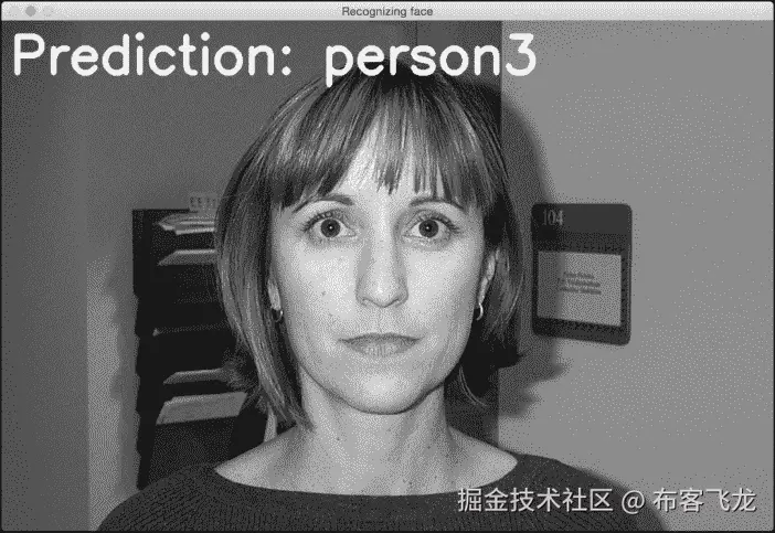
26. The full code is in the face_recognizer.py file that's already provided to you for reference. If you run this code, you will get an output window, which displays the predicted outputs for test images. You can press the Space button to keep looping. There are three different people in the test images. The output for the first person looks like the following:

第二个人的输出如下所示:

第三人称的输出如下图所示:
十一、深度神经网络
在本章中,我们将介绍以下食谱:
- 构建感知机
- 构建单层神经网络
- 构建深度神经网络
- 创建矢量量化器
- 为顺序数据分析建立循环神经网络
- 在光学字符识别数据库中可视化字符
- 利用神经网络构建光学字符识别器
简介
我们的大脑真的很擅长识别和认识事物。我们希望机器也能这样做。神经网络是模仿人脑模拟我们学习过程的框架。神经网络旨在从数据中学习并识别潜在的模式。与所有学习算法一样,神经网络处理数字。因此,如果我们想实现任何涉及图像、文本、传感器等的现实世界任务,我们必须先将它们转换成数字形式,然后再将其输入神经网络。我们可以使用神经网络进行分类、聚类、生成和许多其他相关任务。
神经网络由层层的 神经元组成。这些神经元模仿人脑中的生物神经元。每一层基本上都是一组独立的神经元,它们与相邻层的神经元相连。输入层对应于我们提供的输入数据,输出层由我们想要的输出组成。中间的所有图层都称为 隐藏图层。如果我们设计一个具有更多隐藏层的神经网络,那么我们就给它更多的自由来以更高的精度训练自己。
假设我们希望神经网络根据我们的需求对数据进行分类。为了使神经网络相应地工作,我们需要提供标记的训练数据。然后,神经网络将通过优化成本函数来训练自己。这个成本函数是实际标签和来自神经网络的预测标签之间的误差。我们不断迭代,直到误差低于某个阈值。
深层神经网络到底是什么?深度神经网络是由许多隐藏层组成的神经网络。总的来说,这属于深度学习的范畴。这是一个专门研究这些神经网络的领域,这些神经网络由跨多个垂直方向使用的多层组成。
您可以查看神经网络教程,了解更多关于pages.cs.wisc.edu/~bolo/shipy…的信息。在本章中,我们将使用名为神经实验室 的库。在您继续之前,请确保您安装了它。您可以在pythonhosted.org/neurolab/in…找到安装说明。让我们继续看看如何设计和开发这些神经网络。
构建感知器
让我们从感知器开始我们的神经网络冒险。一个感知器是一个执行所有计算的单神经元。这是一个非常简单的模型,但它构成了建立复杂神经网络的基础。这是它的样子:
神经元使用不同的权重组合输入,然后添加一个偏差值来计算输出。这是一个简单的线性方程,将输入值与感知器的输出联系起来。
怎么做…
-
新建一个 Python 文件,导入以下包:
import numpy as np import neurolab as nl import matplotlib.pyplot as plt -
定义一些输入数据及其对应的标签:
# Define input data data = np.array([[0.3, 0.2], [0.1, 0.4], [0.4, 0.6], [0.9, 0.5]]) labels = np.array([[0], [0], [0], [1]]) -
让我们绘制这个数据,看看数据点位于哪里:
# Plot input data plt.figure() plt.scatter(data[:,0], data[:,1]) plt.xlabel('X-axis') plt.ylabel('Y-axis') plt.title('Input data') -
让我们定义一个有两个输入的
perceptron。这个函数还需要我们在输入数据中指定最小值和最大值:# Define a perceptron with 2 inputs; # Each element of the list in the first argument # specifies the min and max values of the inputs perceptron = nl.net.newp([[0, 1],[0, 1]], 1) -
让我们训练感知器。时代的数量指定了通过我们的训练数据集的完整次数。
show参数指定我们希望显示进度的频率。lr参数指定感知器的学习速率。它是算法在参数空间中搜索的步长。如果这个值很大,那么算法可能会移动得更快,但它可能会错过最佳值。如果这个很小,那么算法会达到最优值,但是会很慢。所以这是一个交易;因此,我们选择一个值0.01:# Train the perceptron error = perceptron.train(data, labels, epochs=50, show=15, lr=0.01) -
让我们绘制结果,如下所示:
# plot results plt.figure() plt.plot(error) plt.xlabel('Number of epochs') plt.ylabel('Training error') plt.grid() plt.title('Training error progress') plt.show() -
The full code is given in the
perceptron.pyfile that's already provided to you. If you run this code, you will see two figures. The first figure displays the input data:第二个图显示了训练错误进度:
构建单层神经网络
现在我们知道如何创建感知器,让我们创建一个单层神经网络。单层神经网络由单层中的多个神经元组成。总的来说,我们将有一个输入层、一个隐藏层和一个输出层。
怎么做…
-
新建一个 Python 文件,导入以下包:
import numpy as np import matplotlib.pyplot as plt import neurolab as nl -
我们将使用
data_single_layer.txt文件中的数据。让我们加载这个:# Define input data input_file = 'data_single_layer.txt' input_text = np.loadtxt(input_file) data = input_text[:, 0:2] labels = input_text[:, 2:] -
让我们绘制输入数据:
# Plot input data plt.figure() plt.scatter(data[:,0], data[:,1]) plt.xlabel('X-axis') plt.ylabel('Y-axis') plt.title('Input data') -
让我们提取最小值和最大值:
# Min and max values for each dimension x_min, x_max = data[:,0].min(), data[:,0].max() y_min, y_max = data[:,1].min(), data[:,1].max() -
让我们定义一个在隐藏层有两个神经元的单层神经网络:
# Define a single-layer neural network with 2 neurons; # Each element in the list (first argument) specifies the # min and max values of the inputs single_layer_net = nl.net.newp([[x_min, x_max], [y_min, y_max]], 2) -
训练神经网络直到 50 个纪元:
# Train the neural network error = single_layer_net.train(data, labels, epochs=50, show=20, lr=0.01) -
绘制结果,如下所示:
# Plot results plt.figure() plt.plot(error) plt.xlabel('Number of epochs') plt.ylabel('Training error') plt.title('Training error progress') plt.grid() plt.show() -
让我们在新的测试数据上测试神经网络:
print single_layer_net.sim([[0.3, 4.5]]) print single_layer_net.sim([[4.5, 0.5]]) print single_layer_net.sim([[4.3, 8]]) -
The full code is in the
single_layer.pyfile that's already provided to you. If you run this code, you will see two figures. The first figure displays the input data:第二个数字显示训练错误进度:
您将在您的终端上看到以下内容,指示输入测试点属于哪里:
[[ 0\. 0.]] [[ 1\. 0.]] [[ 1\. 1.]]您可以根据我们的标签验证输出是否正确。
构建深度神经网络
我们现在准备构建一个深度神经网络。深度神经网络由输入层、许多隐藏层和输出层组成。这看起来如下所示:
上图描绘了具有一个输入层、一个隐藏层和一个输出层的多层神经网络。在深度神经网络中,输入层和输出层之间有许多隐藏层。
怎么做…
-
新建一个 Python 文件,导入以下包:
import neurolab as nl import numpy as np import matplotlib.pyplot as plt -
让我们定义参数来生成一些训练数据:
# Generate training data min_value = -12 max_value = 12 num_datapoints = 90 -
该训练数据将由我们定义的函数组成,该函数将转换这些值。我们希望神经网络能够根据我们提供的输入和输出值,自行学习这一点:
x = np.linspace(min_value, max_value, num_datapoints) y = 2 * np.square(x) + 7 y /= np.linalg.norm(y) -
重塑数组:
data = x.reshape(num_datapoints, 1) labels = y.reshape(num_datapoints, 1) -
绘图输入数据:
# Plot input data plt.figure() plt.scatter(data, labels) plt.xlabel('X-axis') plt.ylabel('Y-axis') plt.title('Input data') -
定义一个具有两个隐藏层的深度神经网络,其中每个隐藏层由 10 个神经元组成:
# Define a multilayer neural network with 2 hidden layers; # Each hidden layer consists of 10 neurons and the output layer # consists of 1 neuron multilayer_net = nl.net.newff([[min_value, max_value]], [10, 10, 1]) -
将训练算法设置为 梯度下降(可在https://spin . atomicobject . com/2014/06/24/gradient-down-linear-relationship)了解更多:
# Change the training algorithm to gradient descent multilayer_net.trainf = nl.train.train_gd -
训练网络:
# Train the network error = multilayer_net.train(data, labels, epochs=800, show=100, goal=0.01) -
在训练数据上运行网络查看性能:
# Predict the output for the training inputs predicted_output = multilayer_net.sim(data) -
绘制训练误差:
```py
# Plot training error
plt.figure()
plt.plot(error)
plt.xlabel('Number of epochs')
plt.ylabel('Error')
plt.title('Training error progress')
```
11. 让我们创建一组新的输入,并在这些输入上运行神经网络,看看它的表现:
```py
# Plot predictions
x2 = np.linspace(min_value, max_value, num_datapoints * 2)
y2 = multilayer_net.sim(x2.reshape(x2.size,1)).reshape(x2.size)
y3 = predicted_output.reshape(num_datapoints)
```
12. 绘制输出:
```py
plt.figure()
plt.plot(x2, y2, '-', x, y, '.', x, y3, 'p')
plt.title('Ground truth vs predicted output')
plt.show()
```
13. The full code is in the deep_neural_network.py file that's already provided to you. If you run this code, you will see three figures. The first figure displays the input data:

第二个图显示了训练错误进度:

第三个图形显示神经网络的输出:

您将在终端上看到以下内容:

创建矢量量化器
也可以使用神经网络进行矢量量化。矢量量化是 N 维版本的“四舍五入”。这在计算机视觉、自然语言处理和一般机器学习的多个领域中非常常用。
怎么做…
-
新建一个 Python 文件,导入以下包:
import numpy as np import matplotlib.pyplot as plt import neurolab as nl -
让我们从
data_vq.txt文件加载输入数据:# Define input data input_file = 'data_vq.txt' input_text = np.loadtxt(input_file) data = input_text[:, 0:2] labels = input_text[:, 2:] -
定义一个两层的学习矢量量化 ( LVQ )神经网络。最后一个参数中的数组指定了每个输出的百分比权重(它们的总和应该是 1):
# Define a neural network with 2 layers: # 10 neurons in input layer and 4 neurons in output layer net = nl.net.newlvq(nl.tool.minmax(data), 10, [0.25, 0.25, 0.25, 0.25]) -
训练 LVQ 神经网络:
# Train the neural network error = net.train(data, labels, epochs=100, goal=-1) -
为测试和可视化创建一个值网格:
# Create the input grid xx, yy = np.meshgrid(np.arange(0, 8, 0.2), np.arange(0, 8, 0.2)) xx.shape = xx.size, 1 yy.shape = yy.size, 1 input_grid = np.concatenate((xx, yy), axis=1) -
评估该网格上的网络:
# Evaluate the input grid of points output_grid = net.sim(input_grid) -
定义我们数据中的四个类:
# Define the 4 classes class1 = data[labels[:,0] == 1] class2 = data[labels[:,1] == 1] class3 = data[labels[:,2] == 1] class4 = data[labels[:,3] == 1] -
定义所有这些类的网格:
# Define grids for all the 4 classes grid1 = input_grid[output_grid[:,0] == 1] grid2 = input_grid[output_grid[:,1] == 1] grid3 = input_grid[output_grid[:,2] == 1] grid4 = input_grid[output_grid[:,3] == 1] -
绘制输出:
# Plot outputs plt.plot(class1[:,0], class1[:,1], 'ko', class2[:,0], class2[:,1], 'ko', class3[:,0], class3[:,1], 'ko', class4[:,0], class4[:,1], 'ko') plt.plot(grid1[:,0], grid1[:,1], 'b.', grid2[:,0], grid2[:,1], 'gx', grid3[:,0], grid3[:,1], 'cs', grid4[:,0], grid4[:,1], 'ro') plt.axis([0, 8, 0, 8]) plt.xlabel('X-axis') plt.ylabel('Y-axis') plt.title('Vector quantization using neural networks') plt.show() -
The full code is in the
vector_quantization.pyfile that's already provided to you. If you run this code, you will see the following figure where the space is divided into regions. Each region corresponds to a bucket in the list of vector-quantized regions in the space:

构建用于序列数据分析的循环神经网络
循环神经网络真的很擅长分析序列和时间序列数据。你可以在上了解更多。当我们处理序列和时间序列数据时,我们不能仅仅扩展通用模型。数据中的时间依赖性非常重要,我们需要在模型中考虑这一点。让我们看看如何构建它们。
怎么做…
-
新建一个 Python 文件,导入以下包:
import numpy as np import matplotlib.pyplot as plt import neurolab as nl -
根据输入参数
def create_waveform(num_points): # Create train samples data1 = 1 * np.cos(np.arange(0, num_points)) data2 = 2 * np.cos(np.arange(0, num_points)) data3 = 3 * np.cos(np.arange(0, num_points)) data4 = 4 * np.cos(np.arange(0, num_points)),定义一个函数来创建波形
-
为每个间隔创建不同的振幅,以创建随机波形:
# Create varying amplitudes amp1 = np.ones(num_points) amp2 = 4 + np.zeros(num_points) amp3 = 2 * np.ones(num_points) amp4 = 0.5 + np.zeros(num_points) -
组合数组以创建输出数组。该数据对应于输入,振幅对应于标签:
data = np.array([data1, data2, data3, data4]).reshape(num_points * 4, 1) amplitude = np.array([[amp1, amp2, amp3, amp4]]).reshape(num_points * 4, 1) return data, amplitude -
定义一个函数,将数据通过训练好的神经网络后绘制输出:
# Draw the output using the network def draw_output(net, num_points_test): data_test, amplitude_test = create_waveform(num_points_test) output_test = net.sim(data_test) plt.plot(amplitude_test.reshape(num_points_test * 4)) plt.plot(output_test.reshape(num_points_test * 4)) -
定义
main功能,从创建样本数据开始:if __name__=='__main__': # Get data num_points = 30 data, amplitude = create_waveform(num_points) -
创建具有两层的循环神经网络:
# Create network with 2 layers net = nl.net.newelm([[-2, 2]], [10, 1], [nl.trans.TanSig(), nl.trans.PureLin()]) -
设置每层的初始化函数:
# Set initialized functions and init net.layers[0].initf = nl.init.InitRand([-0.1, 0.1], 'wb') net.layers[1].initf= nl.init.InitRand([-0.1, 0.1], 'wb') net.init() -
训练循环神经网络:
# Training the recurrent neural network error = net.train(data, amplitude, epochs=1000, show=100, goal=0.01) -
计算网络输出的训练数据:
```py
# Compute output from network
output = net.sim(data)
```
11. 绘图训练错误:
```py
# Plot training results
plt.subplot(211)
plt.plot(error)
plt.xlabel('Number of epochs')
plt.ylabel('Error (MSE)')
```
12. 绘制结果:
```py
plt.subplot(212)
plt.plot(amplitude.reshape(num_points * 4))
plt.plot(output.reshape(num_points * 4))
plt.legend(['Ground truth', 'Predicted output'])
```
13. 创建一个随机长度的波形,看网络能否预测:
```py
# Testing on unknown data at multiple scales
plt.figure()
plt.subplot(211)
draw_output(net, 74)
plt.xlim([0, 300])
```
14. 创建另一个较短长度的波形,看网络能否预测:
```py
plt.subplot(212)
draw_output(net, 54)
plt.xlim([0, 300])
plt.show()
```
15. The full code is in the recurrent_network.py file that's already provided to you. If you run this code, you will see two figures. The first figure displays training errors and the performance on the training data:

第二幅图显示了一个经过训练的循环神经网络如何在任意长度的序列上运行:

您将在您的终端上看到以下内容:

在光学字符识别数据库中可视化字符
我们将现在看看如何使用神经网络来执行光学字符识别。这是指识别图像中手写字符的过程。我们将使用ai.stanford.edu/~btaskar/oc…提供的数据集。下载后的默认文件名为letter.data。首先,让我们看看如何与数据交互并可视化它。
怎么做…
-
新建一个 Python 文件,导入以下包:
import os import sys import cv2 import numpy as np -
定义输入文件名:
# Load input data input_file = 'letter.data' -
定义可视化参数:
# Define visualization parameters scaling_factor = 10 start_index = 6 end_index = -1 h, w = 16, 8 -
继续循环浏览文件,直到用户按下 Esc 键。将该行拆分为制表符分隔的字符:
# Loop until you encounter the Esc key with open(input_file, 'r') as f: for line in f.readlines(): data = np.array([255*float(x) for x in line.split('\t')[start_index:end_index]]) -
将数组重塑为所需的形状,调整其大小,并显示:
img = np.reshape(data, (h,w)) img_scaled = cv2.resize(img, None, fx=scaling_factor, fy=scaling_factor) cv2.imshow('Image', img_scaled) -
如果用户按下 Esc ,中断循环:
c = cv2.waitKey() if c == 27: break -
The full code is in the
visualize_characters.pyfile that's already provided to you. If you run this code, you will see a window displaying characters. For example, o looks like the following:字符 i 看起来如下:
利用神经网络构建光学字符识别器
现在我们知道了如何与数据交互,让我们构建一个基于神经网络的光学字符识别系统。
怎么做…
-
新建一个 Python 文件,导入以下包:
import numpy as np import neurolab as nl -
定义输入文件名:
# Input file input_file = 'letter.data' -
当我们使用处理大量数据的神经网络时,需要花费大量时间进行训练。为了演示如何构建这个系统,我们将只取
20数据点:# Number of datapoints to load from the input file num_datapoints = 20 -
如果您查看数据,您会发现前 20 行中有七个不同的字符。让我们定义它们:
# Distinct characters orig_labels = 'omandig' # Number of distinct characters num_output = len(orig_labels) -
我们将使用 90%的数据进行培训,其余 10%用于测试。定义训练和测试参数:
# Training and testing parameters num_train = int(0.9 * num_datapoints) num_test = num_datapoints - num_train -
数据集文件每行的开始和结束索引:
# Define dataset extraction parameters start_index = 6 end_index = -1 -
创建数据集:
# Creating the dataset data = [] labels = [] with open(input_file, 'r') as f: for line in f.readlines(): # Split the line tabwise list_vals = line.split('\t') -
添加错误检查,查看字符是否在我们的标签列表中:
# If the label is not in our ground truth labels, skip it if list_vals[1] not in orig_labels: continue -
提取标签,并将其附加到主列表中:
# Extract the label and append it to the main list label = np.zeros((num_output, 1)) label[orig_labels.index(list_vals[1])] = 1 labels.append(label) -
提取字符,并将其附加到主列表中:
```py
# Extract the character vector and append it to the main list
cur_char = np.array([float(x) for x in list_vals[start_index:end_index]])
data.append(cur_char)
```
11. 一旦我们有足够的数据就退出循环:
```py
# Exit the loop once the required dataset has been loaded
if len(data) >= num_datapoints:
break
```
12. 将该数据转换为 NumPy 数组:
```py
# Convert data and labels to numpy arrays
data = np.asfarray(data)
labels = np.array(labels).reshape(num_datapoints, num_output)
```
13. 提取我们数据中的维数:
```py
# Extract number of dimensions
num_dims = len(data[0])
```
14. 训练神经网络直到10,000时期:
```py
# Create and train neural network
net = nl.net.newff([[0, 1] for _ in range(len(data[0]))], [128, 16, num_output])
net.trainf = nl.train.train_gd
error = net.train(data[:num_train,:], labels[:num_train,:], epochs=10000,
show=100, goal=0.01)
```
15. 预测测试输入的输出:
```py
# Predict the output for test inputs
predicted_output = net.sim(data[num_train:, :])
print "\nTesting on unknown data:"
for i in range(num_test):
print "\nOriginal:", orig_labels[np.argmax(labels[i])]
print "Predicted:", orig_labels[np.argmax(predicted_output[i])]
```
16. The full code is in the ocr.py file that's already provided to you. If you run this code, you will see the following on your Terminal at the end of training:

神经网络的输出如下图所示:

