CHAPTER 4 The Innovations Process

在许多应用中，这些随机变量具有其他结构，例如，它们可能是由随机过程产生的，如在Ch.1。

尤其是，当随机变量来自一个索引族，即它们是随机过程时，观察到的随机变量的数量可能非常大。在这样的问题中，计算和数据存储方面的考虑都促使我们在随机过程中寻找其他结构，这将减少使用该结构时求解正规方程所需的大量工作。

在本章中，我们将使用几何公式，采用如此创新的方法或新的信息化方法将有助于我们尝试利用其他结构的存在。

4.2基本但简单的观察结果是，当我们具有“子空间的正交基”时，“线性子空间上的投影”特别容易计算

4.2.5;4.3阐明这种观点的价值

4.3将创新技术应用于Ch2的确定性最小二乘问题，将直接导出Sec2.5的array algorithm(QR方法 )。

4.4但是，除非我们能够理解如何识别和利用问题中的特殊结构，否则无论我们是否使用创新，计算的数量都是相同的，而且非常高。

Ch.5引入的“状态空间模型”则可以解决计算量的问题

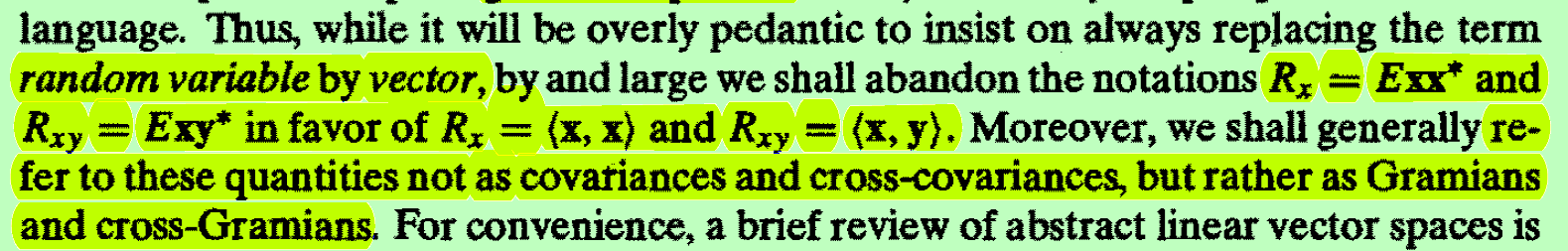
App.4.A为了促进我们的结果更广泛的适用性，我们将经常使用向量和Gramian格拉姆矩阵（而不是过于花哨的词），而不是使用随机变量和协方差矩阵。

4.1 随机过程的估计（ESTIMATION OF STOCHASTIC PROCESSES）

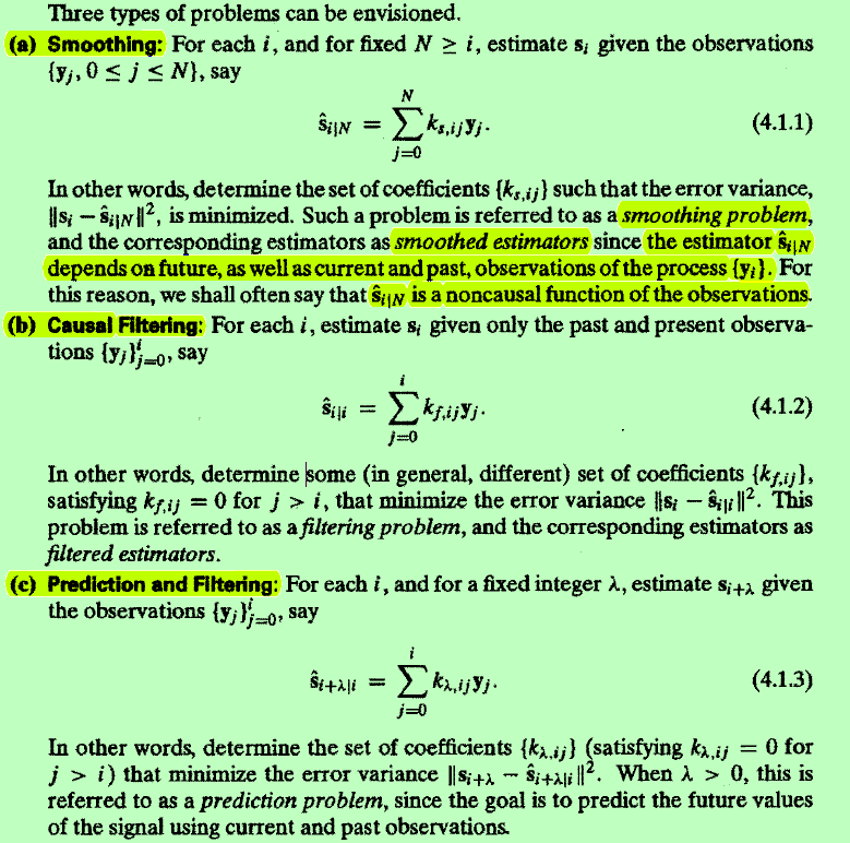
对随机过程的估计有如下三类问题:

smoothing problem:用过去、现在、将来的观察值来估计当下的signal，无因果关系，可以用之前章节的方法来解决
filtering problems:估计量是观察结果的因果函数，用过去、现在的观察值来估计当下的signal
prediction problems:用现在、过去的观测值去估计signal的未来值

对于控制系统而言，状态估计问题是一个动态估计问题，分为三种不同的类型。

如果利用直到当前时刻的实时信息对当前的状态进行估计，称之为滤波问题;

如果利用直到当前时刻的实时信息对未来的状态进行估计，称之为预测问题；

如果利用直到当前时刻的实时信息对过去的状态进行估计，称之为平滑问题。

4.1.1固定间隔Smoothing Problem（The Fixed Interval Smoothing Problem）

从 "观测随机过程" 去估计 "过去的一个未知的随机过程"，可以理解为从一个随机过程的所有随机变量的线性组合去估计未知随机过程的每一个随机变量：

\hat{\mathbf{s}}_{i | N}=\sum_{j=0}^{N} k_{s, i j} \mathbf{y}_{j}?, for each$s_{i}$

将随机过程视为vector，随机过程的随机变量视为vector的元素，如下图所示：

?\mathbf{s}=\operatorname{col}\left\{\mathbf{s}_{0}, \mathbf{s}_{1}, \ldots, \mathbf{s}_{N}\right\}, \quad \hat{\mathbf{s}}_{s}=\operatorname{col}\left\{\hat{\mathbf{s}}_{0 | N}, \hat{\mathbf{s}}_{1 | N}, \ldots, \hat{\mathbf{s}}_{N | N}\right\}, \quad \mathbf{y}=\operatorname{col}\left(\mathbf{y}_{0}, \mathbf{y}_{1}, \ldots, \mathbf{y}_{N}\right\}

然后就有正交条件如下：(error 正交于投影分量)

\left(s_{i}-\sum_{j=0}^{N} k_{s, i j} \mathbf{y}_{j}\right) \perp \mathbf{y}_{l}, \quad \text { for } l=0, \ldots N

然后根据第三章的内容，定义Smoothing Problem自己的inner product：

R_{s y}(i, l)=\sum_{j=0}^{N} k_{s, i j} R_{y}(j, l), \quad \text { for } l=0, \dots N

\begin{aligned}
&\left[R_{s y}(i, 0) \ldots R_{s y}(i, N)\right]=\left[k_{s, i 0} \ldots k_{s, i N}\right] R_{y}\\
&\text { where } R_{y}=\left[R_{y}(i, j)\right]_{i, j=0}^{N}
\end{aligned}

\boldsymbol{R}_{s y} \triangleq\left[\boldsymbol{R}_{s y}(i, j)\right]_{i, j=0}^{N}, \quad \boldsymbol{K}_{s} \triangleq\left[\boldsymbol{k}_{s, i j}\right]_{i, j=0}^{N}

然后直接套上第三章的结论得到以下最优估计：

$\hat{\mathbf{s}}_{s}=K_{s} \mathbf{y} \quad$ and $\quad K_{s} R_{y}=R_{s y}$ or when $R_{y}>0$ $\hat{\mathbf{s}}_{s}=R_{s y} R_{y}^{-1} \mathbf{y}=\langle\mathbf{s}, \mathbf{y}\rangle\langle\mathbf{y}, \mathbf{y}\rangle^{-1} \mathbf{y}$

4.1.2 因果Filtering Problem（The causal Filtering Problem）

与4.1.1类似，但是由于是具有“因果性”，所以矩阵K要求是一个下三角矩阵(j>i则k=0)：

\hat{\mathbf{s}}_{f} \triangleq\left[\begin{array}{c}
\hat{\mathbf{s}}_{0 | \mathbf{0}} \\
\hat{\mathbf{s}}_{111} \\
\vdots \\
\hat{\mathbf{s}}_{N | N}
\end{array}\right]=\left[\begin{array}{cccc}
k_{f, 00} & & \\
k_{f, 10} & k_{f, 11} & & \\
\vdots & & \ddots & \\
k_{f, N 0} & k_{f, N 1} & \dots & k_{f, N N}
\end{array}\right]\left[\begin{array}{c}
\mathbf{y}_{1} \\
\mathbf{y}_{1} \\
\vdots \\
\mathbf{y}_{N}
\end{array}\right]=K_{f} \mathbf{y}

normal function 为如下：

定义一个操作符?\left[(A){\text {lower }}\right]{i j}=\left{\begin{array}{ll} 0 & i<j \ A_{i j} & i \geq j \end{array}\right.?

\left\{R_{s y}-K_{f} R_{y}\right\}_{\text {lower }}=0

meaning：“这个normal function只在下三角区域成立。”

矩阵K要求是一个一个下三角矩阵这一严苛的要求使得normal function难以求解。不过有一个方法Wiener-Hopf integral equation可以解决这个问题。

4.1.3 The Wiener-Hopf Technique

对于这个causal filtering问题的normal function，如何求解出系数矩阵 $K_{f}$ 是本节要探讨的问题。

上式等同于：?K_{f} R_{y}-R_{s y}=U^{+}?， $U^{+}$ 是一个未知的上三角矩阵，因为下三角部分都为0所以满足normal function。

引入LDL(lower×diagonal×lower)分解：

化简normal function:

\underbrace{K_{f} L}_{\text {lower }}=\underbrace{R_{s y} L^{-*} R_{e}^{-1}}_{\text {mixed }}+\underbrace{U^{+} L^{-*} R_{e}^{-1}}_{\text {strictly upper }}

成功解出 $K_{f}$ !:

\boldsymbol{K}_{f}=\left\{R_{s y} L^{-*} \boldsymbol{R}_{e}^{-1}\right]_{\text {lower }} L^{-1}

总结为以下定理：

Lemma 4.1.1 (Optimal Causal Filter) The optimal coefficient matrix $K_{f}$ in $(4.1 .11)$ that solves the causal filtering problem (4.1.2) (or, equivalently, (4.1.8)) is given by

K_{f}=\left\{R_{s y} L^{-*} R_{e}^{-1}\right\}_{\text {lower }} L^{-1}

举了一个例子的两种问题的解法:

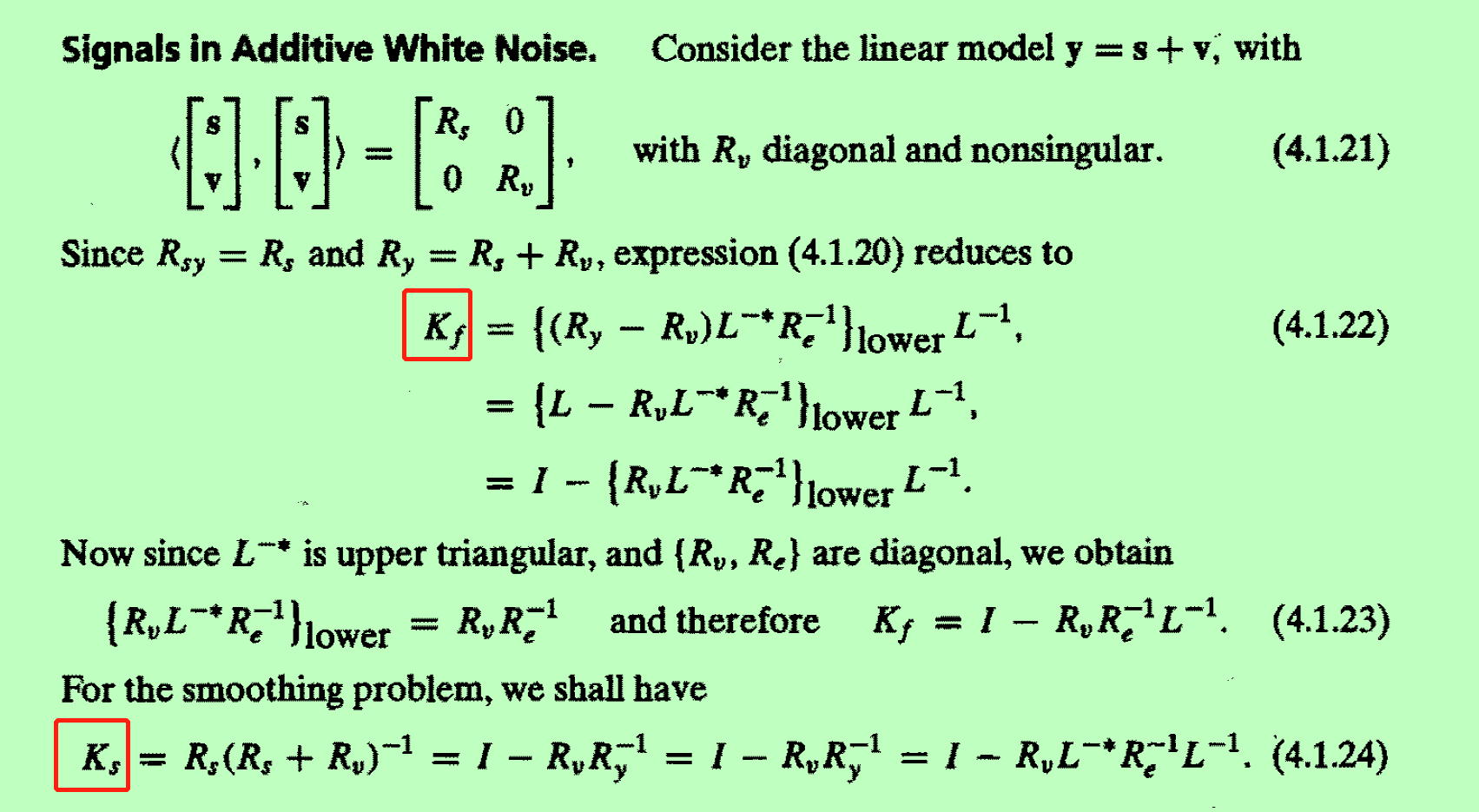
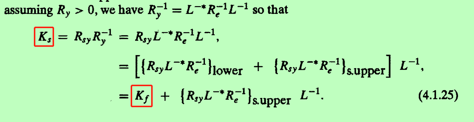
relationship of causal filtering and smoothing problem:

计算量分析：

我们已经看到，解决滤波问题的关键是协方差矩阵R的三角分解。在概念上更简单的平滑问题中，我们所需要的只是矩阵Ry的求逆，或者至少是具有系数矩阵Ry的某些线性方程组的解。实际上，三角分解，矩阵求逆，线性方程组的求解基本上都需要进行相同数量的计算：O（N3）复杂度。而且，三角分解也被证明是矩阵求逆和线性方程解的有用步骤。在接下来的几节中将阐明其成立的原因，我们还将开始探讨如何通过利用问题中的其他结构来减少所需计算量的问题。

4.1.4 A Note on Terminology- Vectors and Gramians

术语替换：

4.2 THE INNOVATIONS PROCESS

C2、C3、C4.1的 least-squares problems 有两个方面值得我们注意：

运算量
数据存储问题：sequential or recursive method解方程

当sequential or recursive method解方程解决后，我们要考虑的就是寻找特殊的structure来减少运算量了：通过algebraic or geometric methods，就是下面几节所要介绍的：

4.2.1 A Geometric Approach

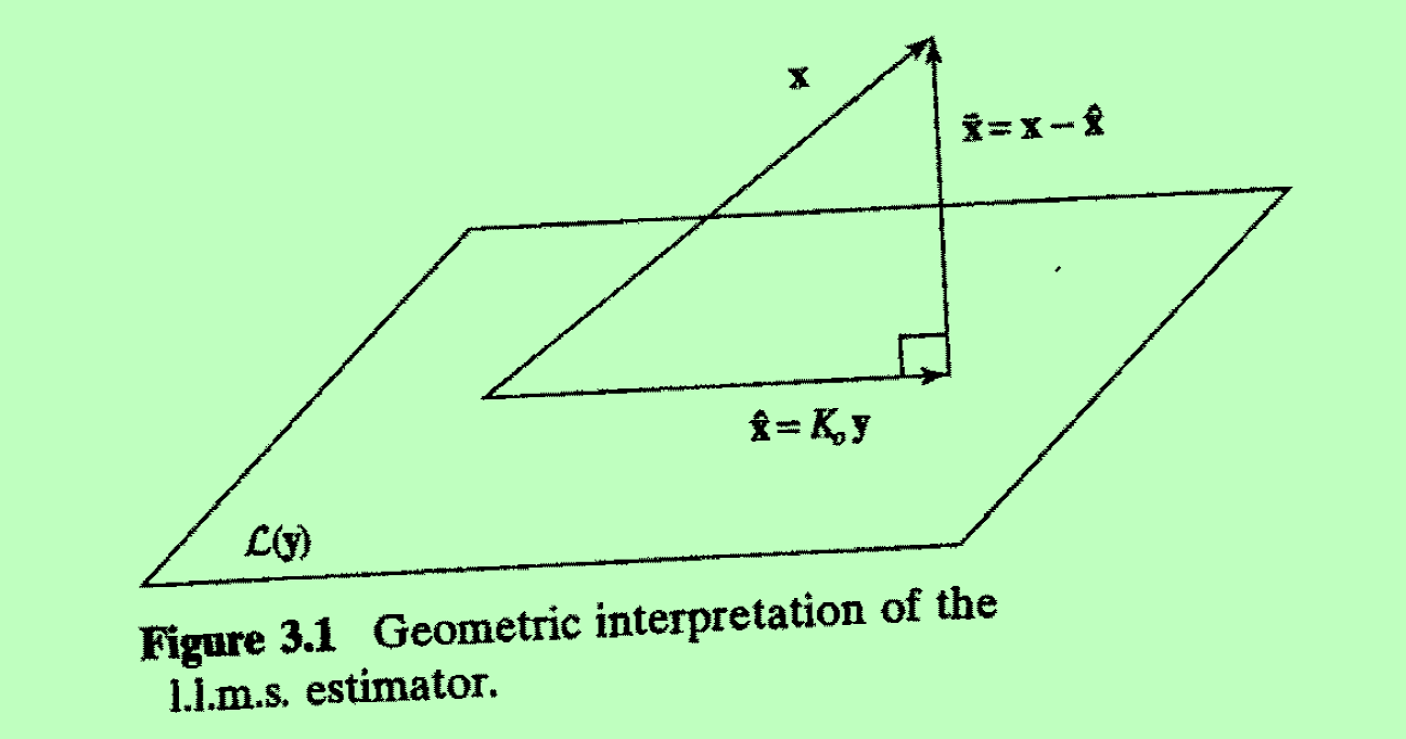
回顾 随机性最小二乘问题 的几何观点：将 $x$ 投影到 $\{y_{1},y_{2},...,y_{N}\}$ 得到最小二乘估计 $\hat{x}$ 。

考虑如果 $R_{y}$ 是一个对角矩阵 == $\{y_{1},y_{2},...,y_{N}\}$ 中都为正交向量，这样的话，x投影到空间中 $\hat{x}$ 就可以由x投影到每一个向量的分量的求和来得到(??不是正交向量就不能这样做吗??)

这样的话如果获得了new information，即 $\{y_{1},y_{2},...,y_{N}\}$ 要添加一个新向量，只需将它正交化即可，然后x投影到它的分量和原先 $\hat{x}$ 直接求和就行。

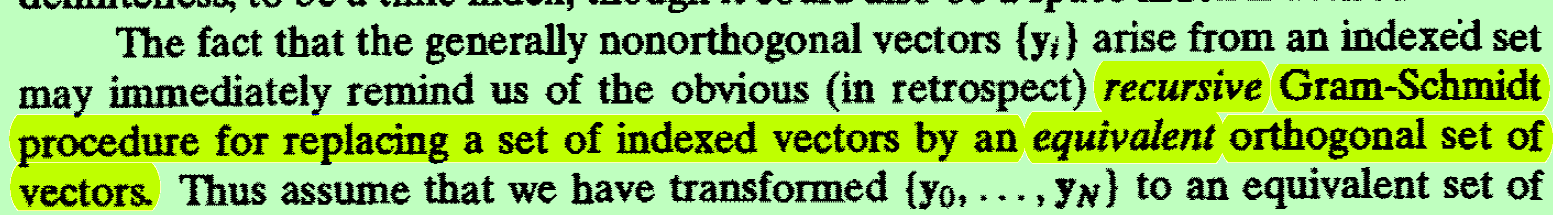
如果 $\{y_{1},y_{2},...,y_{N}\}$ 互相不正交，那么我们就对投影线性空间的所有向量进行 施密特正交化 处理，用的是 recursive Gram-Schmidt procedure：

正交化后结果：

$\mathcal{L}\left\{\mathbf{e}_{0}, \ldots, \mathbf{e}_{N}\right\}=\mathcal{L}\left\{\mathbf{y}_{0}, \ldots, \mathbf{y}_{N}\right\} \triangleq \mathcal{L}_{N}$

若要添加new information：则用recursive Gram-Schmidt procedure:

$\left.\mathbf{e}_{N+1}=\mathbf{y}_{N+1}-\mathbf{P r o j . \{ y}_{N+1} | \mathcal{L}_{N}\right\}$

即 $\mathbf{e}_{N+1}=\mathbf{y}_{N+1}-\sum_{j=0}^{N}\left\langle\mathbf{y}_{N+1}, \mathbf{e}_{j}\right\rangle\left\|\mathbf{e}_{j}\right\|^{-2} \mathbf{e}_{j}$

若 $\{y_{i}\}$ 是很多的随机变量:我们的投影定义为l.l.m.s估计量，error vector就是我们对yn+1的正交化处理后得到的结果，他和原先所有的投影分量(l.l.m.s估计量)垂直

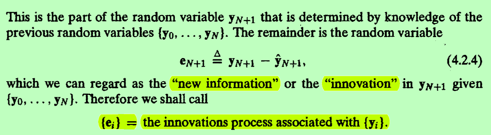
the innovations process is a white-noise process.(见补充知识)(各个分量都是不相关的，就如上面的正交矩阵一样。)

？？4.2.2 An Algebraic Approach

本节应该讲的是用代数的方法来得出4.2.1的结论；并且还将4.2.1的recursive Gram-Schmidt procedure给用矩阵形式包装了一番: $y=Le$

我将看懂的部分来串一串：

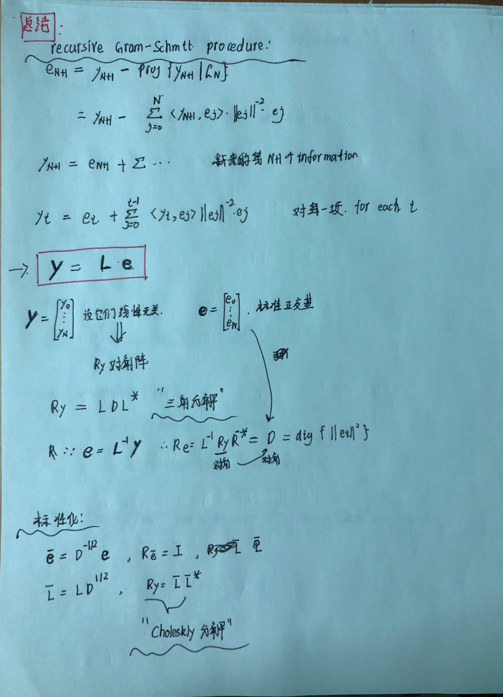
where $L=$

\left[\begin{array}{cccc}
I & & & \\
\left\langle y_{1}, e_{0}\right\rangle|| e_{0}||^{-2} & I & & \\
\left\langle y_{2}, e_{0}\right\rangle|| e_{0}||^{-2} & \left\langle y_{2},\right. & \left.e_{1}\right\rangle|| e_{1}||^{-2} & I \\
\vdots & \vdots & \vdots & \ddots \\
\left\langle y_{N},\right. & \left.e_{0}\right\rangle|| e_{0}||^{-2} & \left\langle y_{N}, e_{1}\right\rangle|| e_{1}||^{-2} & \left(y_{N}, e_{2}\right\rangle|| e_{2}||^{-2} & \ldots
\end{array}\right]

4.2.3 The Modified Gram-Schmidt Procedure

Modified Gram-Schmidt (MGS)正交化法是利用已有正交基计算新的正交基:

(a) Set $e_{0}=y_{0}$ (b) Form $\tilde{\mathbf{y}}_{i | 0}=\mathbf{y}_{i}-\left\langle\mathbf{y}_{i}, \mathbf{e}_{0}\right\rangle\left\|\mathbf{e}_{0}\right\|^{-2} \mathbf{e}_{0},$ and then set $\mathbf{e}_{1}=\tilde{\mathbf{y}}_{110}$ (c) Form $\tilde{\mathbf{y}}_{i 11}=\tilde{\mathbf{y}}_{i 10}-\left\langle\tilde{\mathbf{y}}_{i 0}, \mathbf{e}_{1}\right\rangle\left\|\mathbf{e}_{1}\right\|^{-2} \mathbf{e}_{1},$ and then set $\mathbf{e}_{2}=\tilde{\mathbf{y}}_{211}$ and so on. The partial residuals $\left\{\mathbf{y}_{i}, \tilde{\mathbf{y}}_{i 0}, \tilde{\mathbf{y}}_{i 1}, \ldots\right\}$ can be rearranged in a triangular array, the diagonal entries of which are the innovations $\left\{e_{i}\right\}:$ $\mathbf{y}_{0}$ $\mathbf{y}_{1} \quad \tilde{\mathbf{y}}_{10}$ $\begin{array}{lll}\mathbf{y}_{2} & \tilde{\mathbf{y}}_{2 | 0} & \tilde{\mathbf{y}}_{2 | 1}\end{array}$ $\mathbf{y}_{N} \quad \tilde{\mathbf{y}}_{N | 0} \tilde{\mathbf{y}}_{N | 1} \ldots \tilde{\mathbf{y}}_{N | N-1}$

Now it can be shown that the $i$ -th column of $L(i=0,1, \ldots, N)$ is obtained by taking the inner product of the $i$ -th column in the above table with $\left\|\mathbf{e}_{i}\right\|^{-2} \mathbf{e}_{i}$ (the normalized top entry in that column).

♥4.2.4 Estimation Given the Innovations Process

$\{e_{i}\}$ 就是 Innovations Process

寻找Innovations Process的原因：

We recall that the reason for seeking to determine the innovations is that we can then replace the problem of estimation given the process $\left\{y_{i}, i \leq k\right\}$ , with the simpler one of estimation given the orthogonal innovations process $\left\{e_{i}, i \leq k\right\} .$ Thus

$\hat{\mathbf{x}}_{| N} \triangleq$ the $1.1 . \mathrm{m} . \mathrm{s}$ estimator of $\mathbf{x}$ given $\left\{\mathbf{y}_{0}, \ldots, \mathbf{y}_{N}\right\}$ can also be expressed as

\hat{\mathbf{x}}_{| N}=\text { the l.l.m.s. estimator of } \mathbf{x} \text { given }\left\{\mathbf{e}_{0}, \ldots, \mathbf{e}_{N}\right\}

which, due to the orthogonality of the $\left\{e_{j}\right\}$ , is given by

\hat{\mathbf{x}}_{| N}=\sum_{j=0}^{N}\left\langle\mathbf{x}, \mathbf{e}_{j}\right\rangle\left\|\mathbf{e}_{j}\right\|^{-2} \mathbf{e}_{j}

♥出现新的observation $y_{N+1}$ 后，则先把 $y_{N+1}$ 进行Gram-Schmidt处理得到标准正交基 $e_{N+1}$ ，然后，新的估计量就是原来的估计量加上true value在 $e_{N+1}$ 上的投影：

$\mathbf{e}_{N+1}=\mathbf{y}_{N+1}-\hat{\mathbf{y}}_{N+1 | N}=\mathbf{y}_{N+1}-\sum_{j=0}^{M}\left\langle\mathbf{y}_{N+1} \mathbf{e}_{j}\right\rangle\left\|\mathbf{e}_{j}\right\|^{-2} \mathbf{e}_{j}, \quad \mathbf{e}_{0}=\mathbf{y}_{0}$

\begin{aligned}
\hat{\mathbf{x}}_{| N+1} &\left.=\hat{\mathbf{x}}_{i N}+\text { (1.1.m.s.e. of } \mathbf{x} \text { given } \mathbf{e}_{N+1}\right) \\
&=\hat{\mathbf{x}}_{| N}+\left\langle\mathbf{x}, \mathbf{e}_{N+1}\right\rangle\left\|\mathbf{e}_{N+1}\right\|^{-2} \mathbf{e}_{N+1}, \quad \hat{\mathbf{x}}_{1-1}=0
\end{aligned}

我们可以将这个innovations method用到the filtering problem of Sec. 4.1.2（之前用Wiener-Hopf technique解决），就是下一节要讲的内容。

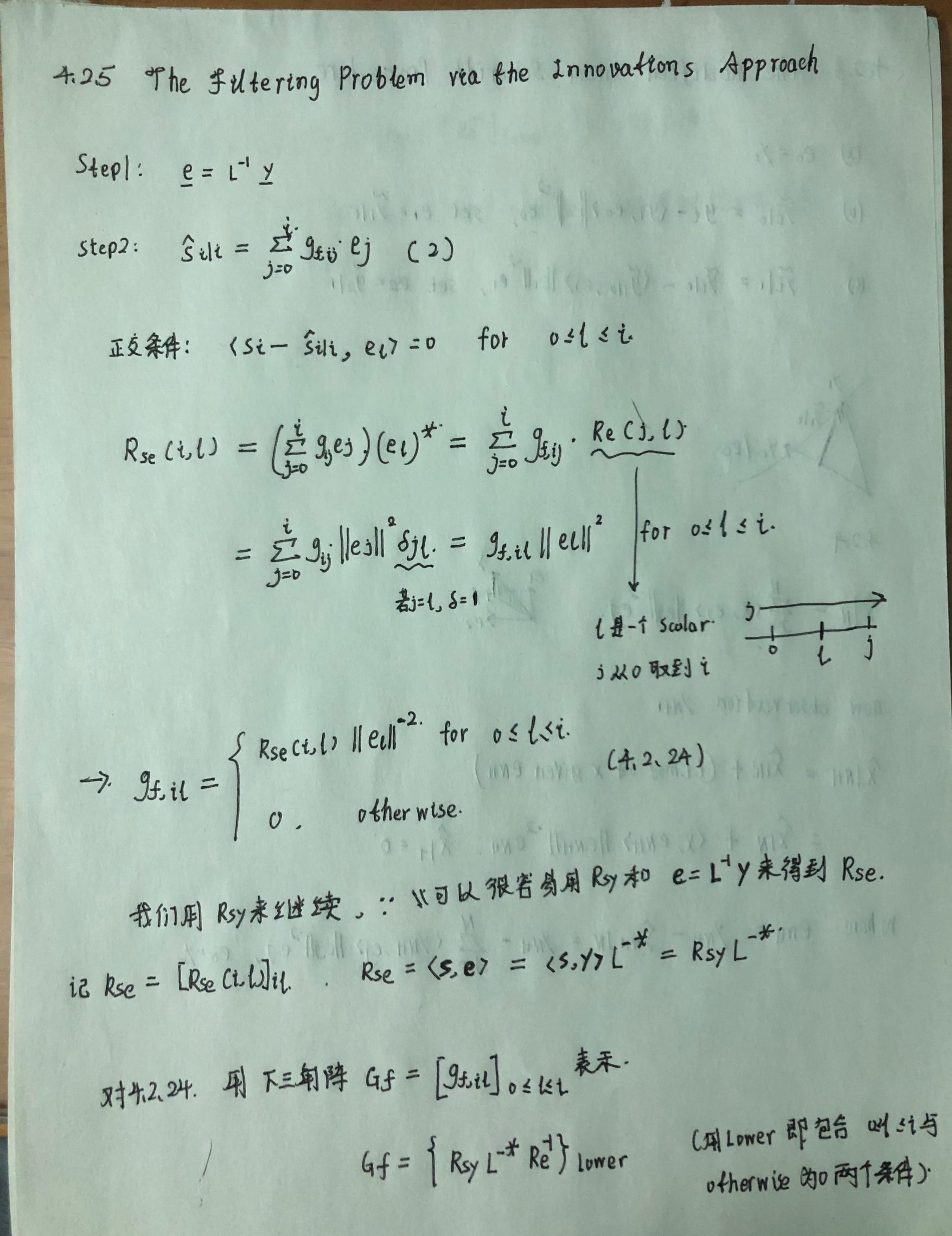
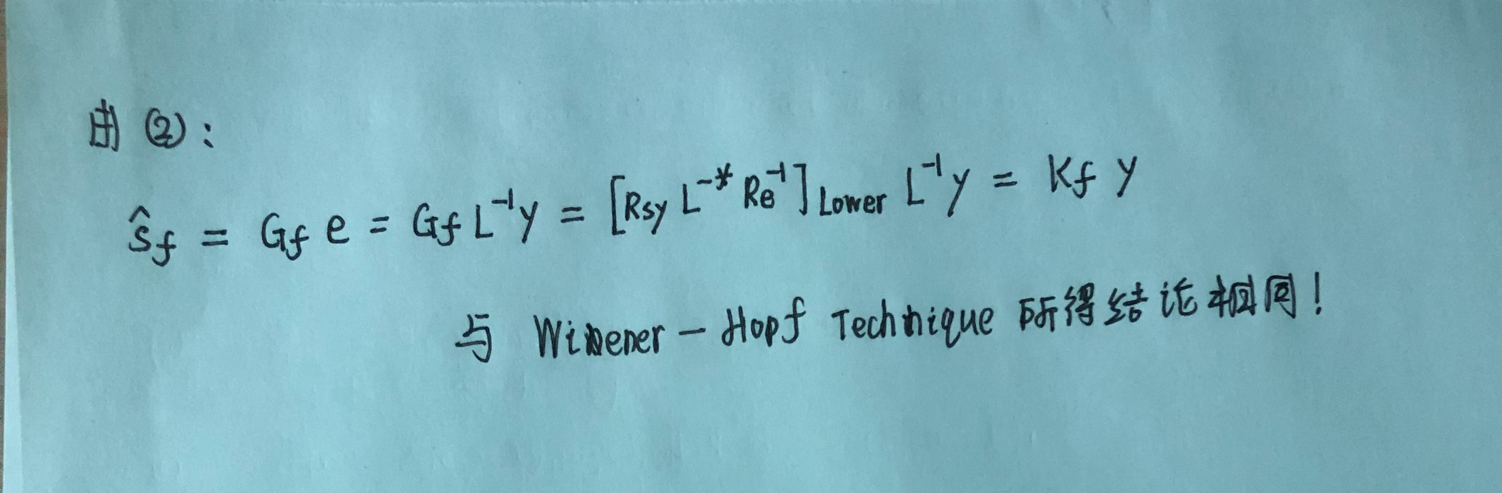
4.2.5 The Filtering Problem via the Innovations Approach

使用innovations approach来解决causal filtering problems，可以完全替代The Wiener-Hopf Technique。更简便，更易懂！

从observation $\{y_{i}\}$ 来估计 $\{s_{i|i}\}$ 整个过程只需要两步

(i) finding the innovations $\left\{e_{i}\right\}$ from the observations $\left\{y_{i}\right\},$

$(\text { ii })$ finding the estimators $\left\{\hat{\mathbf{s}}_{i | i}\right\}$ from the innovations. The second step is easy because the innovations are a white noise process

具体推导过程如下：

4.2.6 Computational Issues

在上述提到的问题中，选择直接对 $R_{y}$ 求逆或者用innovations approach来解决具有相同的复杂度 $O(N^{3})$ ，那innovations approach有啥用捏？

对于一些特殊结构问题（stationarity of the process or the availability of state-space or difference equation models for it,），innovations approach可以减少计算量！

在本书我们主要关注 state-space structure ，用innovations approach可以减少计算量，具体例子如下：

In this book our focus shall be on state-space structure. If we have an $n$ -dimensional state-space model for the process $\left\{y_{i}\right\}$ , then it turns out that the innovations can be found with $O\left(N n^{3}\right)$ operations (see Ch. 9 ), which can be very much less than $O\left(N^{3}\right)$ if $n \ll N$ . Processes with constant parameter state-space models do have displacement structure, and displacement rank $r \leq n ;$ for such processes we shall only need $O\left(N n^{2} r\right)$ operations (see Ch. 11 ). We shall slowly build up to these results. We shall also illustrate many of the points of this section by studying a simple example in Sec. 4.4.

4.3 确定性最小二乘问题的Innovations approach （INNOVATIONS APPROACH TO DETERMINISTIC LEAST-SQUARES PROBLEMS）

Most of our discussions so far have been in terms of random variables regarded as vectors. However as noted several times already, the discussion can often be applied to vectors in any linear space.So, as an example, here we shall consider vectors in N -dimensional Euclidean space as arise in the problems studied in Ch. 2:

我们用Innovations approach方法去解决确定性最小二乘问题,发现结果如果将 $\{e_{i}\}$ 标准化后（即矩阵变成正交矩阵），那么结果和Sec. 2.5的QR方法是几乎一样的！

区别：

H.= QR分解 is not usually carried out via the numerically unreliable GS method（一般不用数值解法解）
而Innovations approach可以用数值方法解（更快？更适合计算机解？）

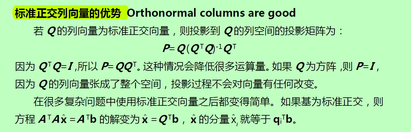
以下为QR分解的好处：（更详细的讨论见Sec. 2.5）

回顾 Ch. 2主要内容：

Most of our discussions so far have been in terms of random variables regarded as vectors. However as noted several times already, the discussion can often be applied to vectors in any linear space. So, as an example, here we shall consider vectors in $N$ -dimensional Euclidean space as arise in the problems studied in Ch. 2

\min _{x}\|y-H x\|^{2}, \quad H \quad \text { full rank }

where $H \in \mathbb{C}^{N \times n},$ the space of possibly complex-valued $N \times n$ matrices, $n \leq N .$ The solution was seen to be (Sec. 2.2)

\hat{x}=\left(H^{*} H\right)^{-1} H^{*} y

which was obtained by projecting $y$ onto the space spanned by the columns $\left(h_{i}\right\}$ of $H$

H=\left[h_{0} \underline{h_{1}} \cdots \underline{h}_{n-1}\right]

现在通过Gram-Schmidt procedure将H变换为各列不相关的矩阵：

$\left[\underline{e}_{0} \underline{e}_{1} \ldots \underline{e}_{n-1}\right]=\left[\begin{array}{lll}h_{0} & \underline{h}_{1} & \ldots & \underline{h}_{n-1}\end{array}\right]\left[\begin{array}{rrr}x & \times & \ldots & x \\ & x & & x \\ & & \ddots & \vdots \\ & & & x\end{array}\right]$

即 $E=H U^{-1}$

Once $E$ and $U$ are found, the solution $\hat{x}$ can be determined by using the condition

\underline{e}_{i}^{*}(y-H \hat{x})=0, \quad i=0,1, \ldots, n-1

E^{*} y=E^{*} H \hat{x}=\left(E^{*} E\right) U \hat{x}

and finally

U \hat{x}=\left(E^{*} E\right)^{-1} E^{*} y

If we normalize the $\left(e_{i}\right\}$ to have unit length, then the decomposition will take the form $H=\hat{Q} \hat{R},$ used in Sec. 2.5 (and in App. A). More explicitly, we can write

H=E U=\underbrace{E\left(E^{*} E\right)^{-* / 2}}_{\hat{Q}} \underbrace{\left(E^{*} E\right)^{* / 2} U}_{\hat{R}}

使用Innovations approach或QR分解的reason：

At least in retrospect, one may ask if we are given $H$ , then why not work directly with $H$ rather than form $H^{*} H$ and then factor it? This is exactly what we do in the innovations approach! The potential numerical benefits of this approach when $H$ is ill-conditioned were explained in Sec. $2.5 .$

4.4 指数相关过程（THE EXPONENTIALLY CORRELATED PROCESS）

举了一个具体的示例来过一遍这一章讲的内容。包括

Ry的三角分解**：**Cholesky factorization 和 LOU （lower-diagonal-upper factorization）
Innovations approach的使用
Gram-Schmidt Procedures的使用：经典法和 modified Gram-Schmidt (MGS) procedure

♥Appendix for Chapter 4 : Linear Spaces, Modules, and Grmians

是对之前Ch. 2 3 4所用到的线性代数知识的补充，包括以下概念：

一

Linear Vector Spaces: $\mathcal{V}$

ring of scalars: $\mathcal{S}$

Inner product space:the triple $\{\mathcal{V}, \mathcal{S},\langle,\rangle\}$ is called an inner product space

module

complex conjugate; conjugate transpose (Hermitian transpose)

二

Gramian Matrices

Gramian Matrices. In the usual mathematical terminology, the Gramian of a collection of vectors $\left\{a_{0}, \ldots, a_{N}\right\}$ (with $a_{i} \in \mathcal{V}$ ) is the matrix

G=\left[\left(a_{i}, a_{j}\right)\right]_{i, j=0}^{N}

By the reflexivity property of the inner product, we can readily see that the Gramian is Hermitian, $G^{*}=G .$ Indeed,

\left[G^{*}\right]_{i j}=\left(G_{j i}\right)^{*}=\left(a_{j}, a_{i}\right)^{*}=\left(a_{i}, a_{j}\right)=G_{i j}

然后讨论了不同问题下的内积定义和 Gramian 矩阵：【n·Dimensional Column Vectors】【n x N Matrices】【Scalar Random Variables】【Vector-Valued Random Variables】

介绍了线性无关的概念，并给出了一个判断线性无关的方法: Gramian test

Definition 4.A.1. (Linear Independence) A set of vectors $x_{i} \in \mathcal{V}, i=0, \ldots, N$ is linearly independent if and only if there exists no set of scalars $\alpha_{i} \in \mathcal{S}, i=0, \ldots, N$ not all identically zero, such that $\sum_{i=0}^{N} \alpha_{i} x_{i}=0$

Lemma 4 A.1 (A Gramian Test) The vectors $\left\{a_{i} \in \mathcal{V}, i=0,1, \ldots, N\right\}$ are linearly independent if, and only if their corresponding Gramian matrix is nonsingular.

之前假设 $R_{y}>0$ 就是让observation $\{y_{i}\}$ 之间线性无关。

确定性最小二乘和随机性最小二乘问题的normal function都用到了Grammian矩阵来当系数矩阵：

$\left(H^{*} H\right) \hat{x}=H^{*} y$ and $K_{o} R_{y}=R_{x y}$

三

linear subspace

basis vectors

orthonormal basis

Lemma $4 . A .2$ (Uniqueness of Projections) Given $y \in \mathcal{V},$ there exists a unique element of $\mathcal{L},$ denoted by $\hat{y},$ such that