Deep Reinforcement Learning For Sequence to Sequence Models

Yaser Keneshloo, Tian Shi, Naren Ramakrishnan, Chandan K. Reddy,  Y. Keneshloo is with the Department of Computer Science at Virginia Tech, Arlington, VA. Corresponding author: yaserkl@vt.edu.T. Shi is with the Department of Computer Science at Virginia Tech, Arlington, VA. Email: tshi@vt.edu.N. Ramakrishnan is with the Department of Computer Science at Virginia Tech, Arlington, VA. Email: naren@cs.vt.edu.C. K. Reddy is with the Department of Computer Science at Virginia Tech, Arlington, VA. Email: reddy@cs.vt.edu.Y. Keneshloo is with the Department of Computer Science at Virginia Tech, Arlington, VA. Corresponding author: yaserkl@vt.edu.T. Shi is with the Department of Computer Science at Virginia Tech, Arlington, VA. Email: tshi@vt.edu.N. Ramakrishnan is with the Department of Computer Science at Virginia Tech, Arlington, VA. Email: naren@cs.vt.edu.C. K. Reddy is with the Department of Computer Science at Virginia Tech, Arlington, VA. Email: reddy@cs.vt.edu.Y. Keneshloo is with the Department of Computer Science at Virginia Tech, Arlington, VA. Corresponding author: yaserkl@vt.edu.T. Shi is with the Department of Computer Science at Virginia Tech, Arlington, VA. Email: tshi@vt.edu.N. Ramakrishnan is with the Department of Computer Science at Virginia Tech, Arlington, VA. Email: naren@cs.vt.edu.C. K. Reddy is with the Department of Computer Science at Virginia Tech, Arlington, VA. Email: reddy@cs.vt.edu.Y. Keneshloo is with the Department of Computer Science at Virginia Tech, Arlington, VA. Corresponding author: yaserkl@vt.edu.T. Shi is with the Department of Computer Science at Virginia Tech, Arlington, VA. Email: tshi@vt.edu.N. Ramakrishnan is with the Department of Computer Science at Virginia Tech, Arlington, VA. Email: naren@cs.vt.edu.C. K. Reddy is with the Department of Computer Science at Virginia Tech, Arlington, VA. Email: reddy@cs.vt.edu.Y. Keneshloo is with the Department of Computer Science at Virginia Tech, Arlington, VA. Corresponding author: yaserkl@vt.edu.T. Shi is with the Department of Computer Science at Virginia Tech, Arlington, VA. Email: tshi@vt.edu.N. Ramakrishnan is with the Department of Computer Science at Virginia Tech, Arlington, VA. Email: naren@cs.vt.edu.C. K. Reddy is with the Department of Computer Science at Virginia Tech, Arlington, VA. Email: reddy@cs.vt.edu.Y. Keneshloo is with the Department of Computer Science at Virginia Tech, Arlington, VA. Corresponding author: yaserkl@vt.edu.T. Shi is with the Department of Computer Science at Virginia Tech, Arlington, VA. Email: tshi@vt.edu.N. Ramakrishnan is with the Department of Computer Science at Virginia Tech, Arlington, VA. Email: naren@cs.vt.edu.C. K. Reddy is with the Department of Computer Science at Virginia Tech, Arlington, VA. Email: reddy@cs.vt.edu.Y. Keneshloo is with the Department of Computer Science at Virginia Tech, Arlington, VA. Corresponding author: yaserkl@vt.edu.T. Shi is with the Department of Computer Science at Virginia Tech, Arlington, VA. Email: tshi@vt.edu.N. Ramakrishnan is with the Department of Computer Science at Virginia Tech, Arlington, VA. Email: naren@cs.vt.edu.C. K. Reddy is with the Department of Computer Science at Virginia Tech, Arlington, VA. Email: reddy@cs.vt.edu.Y. Keneshloo is with the Department of Computer Science at Virginia Tech, Arlington, VA. Corresponding author: yaserkl@vt.edu.T. Shi is with the Department of Computer Science at Virginia Tech, Arlington, VA. Email: tshi@vt.edu.N. Ramakrishnan is with the Department of Computer Science at Virginia Tech, Arlington, VA. Email: naren@cs.vt.edu.C. K. Reddy is with the Department of Computer Science at Virginia Tech, Arlington, VA. Email: reddy@cs.vt.edu. Submitted on 24 May 2018 ArXiV page Original PDF

Abstract

In recent years, sequence-to-sequence (seq2seq) models are used in a variety of tasks from machine translation, headline generation, text summarization, speech to text, to image caption generation. The underlying framework of all these models are usually a deep neural network which contains an encoder and decoder. The encoder processes the input data and a decoder receives the output of the encoder and generates the final output. Although simply using an encoder/decoder model would, most of the time, produce better result than traditional methods on the above-mentioned tasks, researchers proposed additional improvements over these sequence to sequence models, like using an attention-based model over the input, pointer-generation models, and self-attention models. However, all these seq2seq models suffer from two common problems: 1) exposure bias and 2) inconsistency between train/test measurement. Recently a completely fresh point of view emerged in solving these two problems in seq2seq models by using methods in Reinforcement Learning (RL). In these new researches, we try to look at the seq2seq problems from the RL point of view and we try to come up with a formulation that could combine the power of RL methods in decision-making and sequence to sequence models in remembering long memories. In this paper, we will summarize some of the most recent frameworks that combines concepts from RL world to the deep neural network area and explain how these two areas could benefit from each other in solving complex seq2seq tasks. In the end, we will provide insights on some of the problems of the current existing models and how we can improve them with better RL models. We also provide the source code for implementing most of the models that will be discussed in this paper on the complex task of abstractive text summarization.

deep learning; reinforcement learning; sequence to sequence learning; Q-learning; actor-critic methods; policy gradients.

1 Introduction

Sequence to sequence (seq2seq) framework is a common framework for solving sequential problems [1]. In seq2seq models, the input to the model is a sequence of some data units and the output also is a sequence of data units. Traditionally, these models are trained using Teacher Forcing [2] in which the model is trained based on a ground-truth sequence. Recently, there has been various researches to connect learning of these models with Reinforcement Learning (RL) techniques. In this paper, we will summarize some of the recent works in seq2seq training that use RL methods to enhance the performance of these models and talk about various challenges that we face when applying RL methods to train a seq2seq model. We hope that this paper will provide a broad overview on the strength and complexity of combining seq2seq training with RL training and help researchers to choose the right RL algorithm for solving their problem. Section 1.1 will shortly introduce how a simple seq2seq model works and Section 1.2 talks about some of problems of seq2seq models and later on in Section 1.3, we provide an introduction of RL models and explain how these models could solve the problems of seq2seq models and finally in Section 1.4 we provide a roadmap on how this paper is organized and what we will cover throughout the paper.

1.1 Seq2seq Framework

Seq2seq models are common in various applications ranging from 1) machine translation [3, 4, 5, 6, 7, 8], where the input is a sentence (sequence of words) from one language (English) and the output is the translation to another language (French), 2) news headline generation [9, 10], where the input is a news article (sequence of words) or the first two or three sentences of it and the output is the headline of the news, 3) text summarization [11, 12, 13, 14], where the input is a complete article (sequence of words) and output is a short summary of it (sequence of words), 4) speech to text [15, 16, 17, 18], where the input is an audio of a speech (sequence of audibles pieces) and the output is the speech text (sequence of words), 5) image captioning [19, 20, 21], where the input is an image (sequence of different layers of image) and output is a textual caption explaining the image (sequence of words).

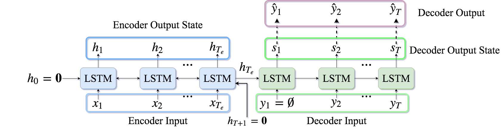
In recent years, the general framework for solving these problems is by using deep neural networks which has two main parts: an encoder which reads the sequence of input data and a decoder which uses the output generated by encoder and produce the sequence of outputs. Fig 1 gives a schematic of this simple framework. The encoder and decoder are usually implemented by Recurrent Neural Networks (RNN) such as LSTM [22]. The encoder takes a sequence of length Te inputs¹, X={x1,x2,⋯,xTe}, where xt∈A={1,⋯,|A|} is a single input coming from a range of possible inputs, A, and generates the output state ht. In addition, each encoder, receives the state of the previous encoder’s hidden state, ht−1, and if the encoder is a bidirectional LSTM, it will also receives the state from the next encoder’s hidden state, ht+1 to generate its current hidden state ht. The decoder, on the other hand, takes the last state from encoder, i.e. hTe and starts generating an output of size T<Te, ^Y={^y1,^y2,⋯,^yT}, based on the current state of the decoder, st and the ground-truth output, yt. The decoder could also take as input an additional context vector ct, which encodes the context to be used while generating the output [6, 9, 3]. The RNN learns a recursive function to compute st and outputs the distribution over the next output:

ht′=Φθ(xt′,ht)st′=Φθ(yt,st/hTe,ct)^yt′∼πθ(y|^yt,st′)

(1)

where t′=t+1, θ is the parameters of the model, and the function for πθ and Φθ depends on the type of RNN. A simple Elman RNN [23] would use Sigmoid function for Φ and Softmax function for π [1]:

st′=σ(W1yt+W2st+W3ct)ot′=Softmax(W4st′+W5ct)

(2)

where ot is the output distribution of size |A| and we select the output ^yt from this distribution. W1, W2, W3, W4, and W5 are matrices of learnable parameters of sizes W1,2,3∈Rd×d and W4,5∈Rd×|A|, where d is the size of the input representation (like size of the word embedding in text summarization). We assume the first decoder input is a special input indicating the beginning of a sequence, denoted by y0=∅ and the first forward hidden state h0 and the last backward hidden state hTe+1 for encoder are set to a zero vector. Moreover, the first hidden state for decoder s0 is set to the output that we receive from the last encoding state, i.e. hTe.

The most widely used method to train the decoder for sequence generation is called Teacher Forcing algorithm [2], which minimizes the maximum-likelihood loss at each decoding step. Let’s define y={y1,y2,⋯,yT} as the ground-truth output sequence for a given input sequence X. The maximum-likelihood training objective is the minimization of the following Cross-Entropy (CE) loss:

LCE=−T∑t=1logπθ(yt|yt−1,st,ct−1,X)

(3)

Once the model is trained with the above objective, we can use the model to generate an entire sequence as follows: Let ^yt denotes the action (output) taken by the model at the time t. Then the next action is generated by:

^yt′=argmaxyπθ(y|^yt,st′)

(4)

This process could be improved by using beam search to find a reasonable good output sequence [7]. Now, given the ground-truth output Y and the model generated output ^Y, we can evaluate the performance of the model with a specific metric. In seq2seq problems, we use discrete measures such as ROUGE [24], BLEU [25], METEOR [26], CIDEr [27] to evaluate the model. For instance, ROUGEl, which is an evaluation metric for textual seq2seq tasks, uses the largest common substring between Y and ^Y to evaluate the goodness of the generated output. Algorithm 1 shows these steps.

Input: Input sequences, X, and ground-truth output sequences, Y. Output: Trained seq2seq model. Training Steps: for batch of input and output sequences X and Y do       Run encoding on X and get the last encoder state, hTe.       Run decoding by feeding hTe to the first decoder and get the       sampled output sequence ^Y.       Calculate the loss according to Eq. (3) and update the parameters       of the model. end for Testing Steps: for batch of input and output sequences X and Y do       Use the trained model and Eq. (4) to sample the output ^Y       Evaluate the model using a performance metric, e.g. ROUGEl end for

1.2 Problems of Seq2seq Models

One of the main issues with current seq2seq models is that minimizing LCE does not always produce the best results on these discrete evaluation metrics. Therefore, using cross-entropy loss for training a seq2seq model creates a mismatch in generating the next action during training and testing. As shown in Fig 1 and also according to Eq. (3), during training, the decoder uses the two inputs, first the previous output state, st−1 and the ground-truth input, yt to calculate its current output state, st and use it to generate the next action, ^yt. While at test-time, Eq. (4), the decoder completely relies on the previously generated action from the model distribution to predict the next action, since the ground-truth data is not available, anymore. Therefore, in summary, during training the input to the decoder is from ground-truth but during test the input come from the model distribution. This exposure bias [28], results in error accumulation during generation at test time, since the model has never been exposed only to its own predictions during training. To avoid the exposure bias problem, we need to remove the ground-truth dependency during training and use only the model distribution to minimize Eq. (3). One way to handle this situation is through the scheduled sampling method [2]. This way, we first pre-train the model using cross-entropy loss and then we slowly replace the ground-truth with a sampled action from the model. Therefore, we randomly decide whether to use the ground-truth action with probability ϵ, or an action coming from the model itself with probability (1−ϵ). When ϵ=1, the model is trained using Eq. (3), while when ϵ=0 the model is trained based on the following loss:

LInference=−T∑t=1logπθ(^yt|^y1,⋯,^yt−1,st,ct−1,X)

(5)

Note that the difference between this equation and CE loss is on the fact that in CE we use the ground-truth output, yt, to calculate the loss while in this equation, we use the output of the model, ^yt to calculate the loss.

Although, scheduled sampling is a simple way to avoid the exposure bias, it does not provide a clear solution for the back-propagation of error and therefore it is statistically inconsistent [29]. Recently, Goyal et al. [30] proposed a solution for this problem by creating a continuous relaxation over the argmax operation to create a differentiable approximation of the greedy search during decoding steps.

The second problem with seq2seq models is that while we train the model using the LCE, we typically evaluated the model during test time using discrete and non-differentiable metrics such as BLEU and ROUGE. This will create a mismatch between the training objective and the test objective and therefore could yield to inconsistent results. Recently, it has been shown that both the exposure bias and non-differentiability of evaluation metrics can be addressed by incorporating techniques from Reinforcement Learning.

1.3 Reinforcement Learning

In RL, we consider a sequential decision making process, in which an agent interacts with an environment \upvarepsilon over discrete time steps t[31]. The goal of the agent is to do a specific job, like moving an object [32, 33], playing Go [34] or an Atari game [35], or picking the best word for the news summary [13, 36]. The idea is that given the environment state at time t is st, the agent picks an action ^yt∈A={1,⋯,|A|}, according to a policy π(^yt|st) and observe a reward rt for that action². For instance, we can consider our seq2seq conditioned RNN as a stochastic policy that generates actions (selecting the next output) and receives the task reward based on a discrete measure like ROUGE as the return. The agent’s goal is to maximize the expected discounted reward, Rt=∑Tτ=tγτ−trτ, where γ∈[0,1] is a discount factor that trades-off the importance of immediate and future rewards. Under the policy π, we can define the values of the state-action pair Q(st,yt) and the state V(st) as follows:

Qπ(st,yt)=E[rt|s=st,y=yt]Vπ(st)=Ey∼π(s)[Qπ(st,y=yt)]

(6)

The preceding state-action function (Q function for short) can be computed recursively with dynamic programming:

Qπ(st,yt)=Est′[rt+γEyt′∼π(st′)[Qπ(st′,yt′)]Vπ(st′)]

(7)

Given above definitions, we can define a function called advantage, relating the value function V and Q function as follows:

Aπ(st,yt)=Qπ(st,yt)−Vπ(st)=rt+γEst′∼π(st′|st)[Vπ(st′)]−Vπ(st)

(8)

where Ey∼π(s)[Aπ(s,y)]=0 and for a deterministic policy, y∗=argmaxyQ(s,y), it follows that Q(s,y∗)=V(s), hence A(s,y∗)=0. Intuitively, the value function V measures how good the model could be when it is in a specific state s. The Q function, however, measures the value of choosing a specific action when we are in such state. Given these two functions, we can obtain the advantage function which captures the importance of each action by subtracting the value of the state, V from the Q function. In practice, we use our seq2seq model as the policy which generates actions. Definition of an action, however will be task-specific meaning that for a text summarization task, action resembles choosing the next token for the summary, while for a question answering task, the action might be defined as the start and end index of the answer in the document. Also, definition of reward function could vary from one application to another. For instance, in text summarization, measures like ROUGE and BLEU are commonly used while in image captioning, CIDEr and METEOR are common. Finally, the state of the model is usually defined as the decoder output state at each time. Therefore, we use the decoder output state at each time as the current state of the model and use it to calculate our Q, V, and advantage function. Table I summarizes the notations used in this paper.

Seq2seq Model Parameters
X	The sequence of input of length Te, X={x1,x2,⋯,xTe}.
Y	The sequence of ground-truth output of length T, Y={y1,y2,⋯,yT}.
^Y	The sequence of output generated by model of length T, ^Y={^y1,^y2,⋯,^yT}.
Te	Length of the input sequence and number of encoders.
T	Length of the output sequence and number of decoders.
d	Size of the input and output sequence representation.
A	Input and output shared vocabulary.
ht	Encoder hidden state at time t.
st	Decoder hidden state at time t.
πθ	The seq2seq model with parameter θ.
Reinforcement Learning Parameters
r(st,yt)=rt	The reward that agent receives by taking the action yt when the state of the environment is st
^Y	Sets of actions that the agent is taking for a period of time T, ^Y={^y1,^y2,⋯,^yT} This is similar to the output that seq2seq model is generating.
π πθ	The policy that agent uses to take the action. In seq2seq models, we use the RNN network with parameter θ as our policy.
γ	Discount factor to reduce the effect of the reward of future actions.
Q(st,yt) Qπ(st,yt)	The Q-value (under policy π) that shows the estimated reward of taking action yt when we are at state st.
QΨ(st,yt)	A function approximator with parameter Ψ that estimates the Q-value given the state-action pair at time t.
V(st) Vπ(st)	Value function which calculate the expectation of Q-value (under policy π) over all possible actions.
VΨ(st)	A function approximator with parameter Ψ that estimates the value function given the state at time t.
Aπ(st,yt)	Advantage function (under policy π) which defines how good a state-action pair is w.r.t the expected reward we can receive at this state.
AΨ(st,yt)	A function approximator with parameter Ψ that estimates the advantage function the state-action pair at time t.

1.4 Paper Organization

In general, we can propose the following simple yet complex problem statement that we are trying to solve by combining these two different models of learning:

Problem Statement: Given a series of input data and a series of ground-truth outputs, train a model that:

• Only relies on its own output, rather than the ground-truth, to generate the results (avoiding exposure bias).

• Directly optimize the model using the evaluation metric (avoiding mismatch between training and test measures).

Although recently there have been two great survey articles on the topic of deep reinforcement learning [37, 38], these articles heavily focus on the reinforcement learning side and their applications in robotic and vision, while they provide less information on how these model could be use in a variety of other tasks. In this paper, we will summarize some of the most recent frameworks that attempted to find a solution for the above problem statement in a broad range of applications and explain how RL and seq2seq learning could benefit from each other in solving complex tasks. In the end, we will provide insights on some of the problems of the current existing models and how we can improve them with better RL models. The goal of this paper is to provide information about how we can broaden the power of seq2seq models with RL methods and understand challenges that exist in applying these methods to the deep learning problems. Also, one of the main issue with current literatures on training seq2seq models with RL method is the lack of a good open-source framework for implementing these ideas. Along with this paper, we have provided a library that focuses on the complex task of abstractive text summarization and combines the state-of-the-art methods in this task with the recent techniques used in deep RL. The library provides a lot of different options and hyperparameters for training the seq2seq model using different RL models. Experimenting over the full capability of this framework takes a lot of computing hours since training each models with a specific configuration requires intense GPU computing. Therefore, we encourage researchers to play around with the hyperparameters and explore how they can use this framework to gain better results on different seq2seq tasks. Therefore, the contribution in this paper could be summarized as follows:

• Provide a comprehensive summary of RL methods that are used in deep learning and specifically in training seq2seq model.

• Provide all the challenges, advantages, and disadvantages of different RL methods that are used in seq2seq training.

• Provide guidelines on how one could improve a specific RL method to get a better and smoother training for seq2seq models.

• Provide an open-source library for implementing a complex seq2seq model using different RL techniques ³.

This paper is organized as follows: Section 3 provides details over some of the common RL techniques used in training seq2seq models. We provide a brief introduction of different seq2seq models in Section 4 and later in Section 4 we explain various RL models that could be used alongside the seq2seq training. We provide a summary of the recent real-world applications that combines RL training with seq2seq training and in Section 5 we talk about the framework that we implemented and how we can use it for different seq2seq problems. Finally, in Section 6 we provide the conclusion of the paper.

2 Seq2seq Models and Their Applications

Sequence to Sequence (seq2seq) models have been an integral part of most of the current real-world problems. From Google Machine Translation [4] to Apple’s Siri speech to text [39], seq2seq models provide a clear framework to process information that are in the form of sequences. In a seq2seq model, the input and output are in the form of sequences of single units like sequence of words, images, or speech units. Table II provides a brief summary of various seq2seq models and their respective input and output. We also provided some of the most important researches regarding each application along with each problem.

Application	Problem Description	Input	Output	References
Machine Translation	Translating a sentence from a source language to a target language	A sentence (sequence of words) in language A (e.g. English)	Another sentence (sequence of words) in language B (e.g. French)	[6, 1, 7, 3, 40]
Text Summarization Headline Generation	Summarizing a document into a more concise and shorter summary	A long document like a news article (sequence of words)	A short summary/headline (sequence of words)	[9, 10, 14, 41] [12, 42, 43]
Question Generation	Generating interesting questions from a text document or an image	A piece of text (sequence of words) or image (sequence of layers)	A set of questions (sequence of words) related to the text or image	[44, 45, 46, 47]
Question Answering	Given a text document or an image and a question, find the answer to the question	A textual question (sequence of words)or an image (sequence of layers)	A single word answer from a document or the start and end index of the answer in the document	[48, 49, 50, 49]
Dialogue Generation	Generate a dialogue between two agents like between a robot and human	A dialogue from the first agent (sequence of words) or audibles (sequence of speech units)	A dialogue from the second agent (sequence of words) or audibles (sequence of speech units)	[51, 52, 53, 54]
Image Captioning	Given an image, generate a caption that explains the content of the image	An image (sequence of layers)	The caption (sequence of words) describing that image	[55, 56, 57, 58] [19, 20, 59]
Video Captioning	Given a video clip, generate a caption that explains the content of the video	A video (sequence of images)	The caption (sequence of words) describing the video	[60, 61, 62, 63]
Computer Vision	Finding interesting events in a video, like predicting the next action of a specific object in the video	A video (sequence of images)	Differs from applications to applications. For instance, we could be interested in figuring out the next action of a specific object or entity in the video	[?, 64, 65, 66]
Speech Recognition	Given a piece of audible input (like a speech), convert it to the text and vice versa	A speech (sequence of speech units)	The text of that speech (sequence of words)	[67, 68, 17, 16]

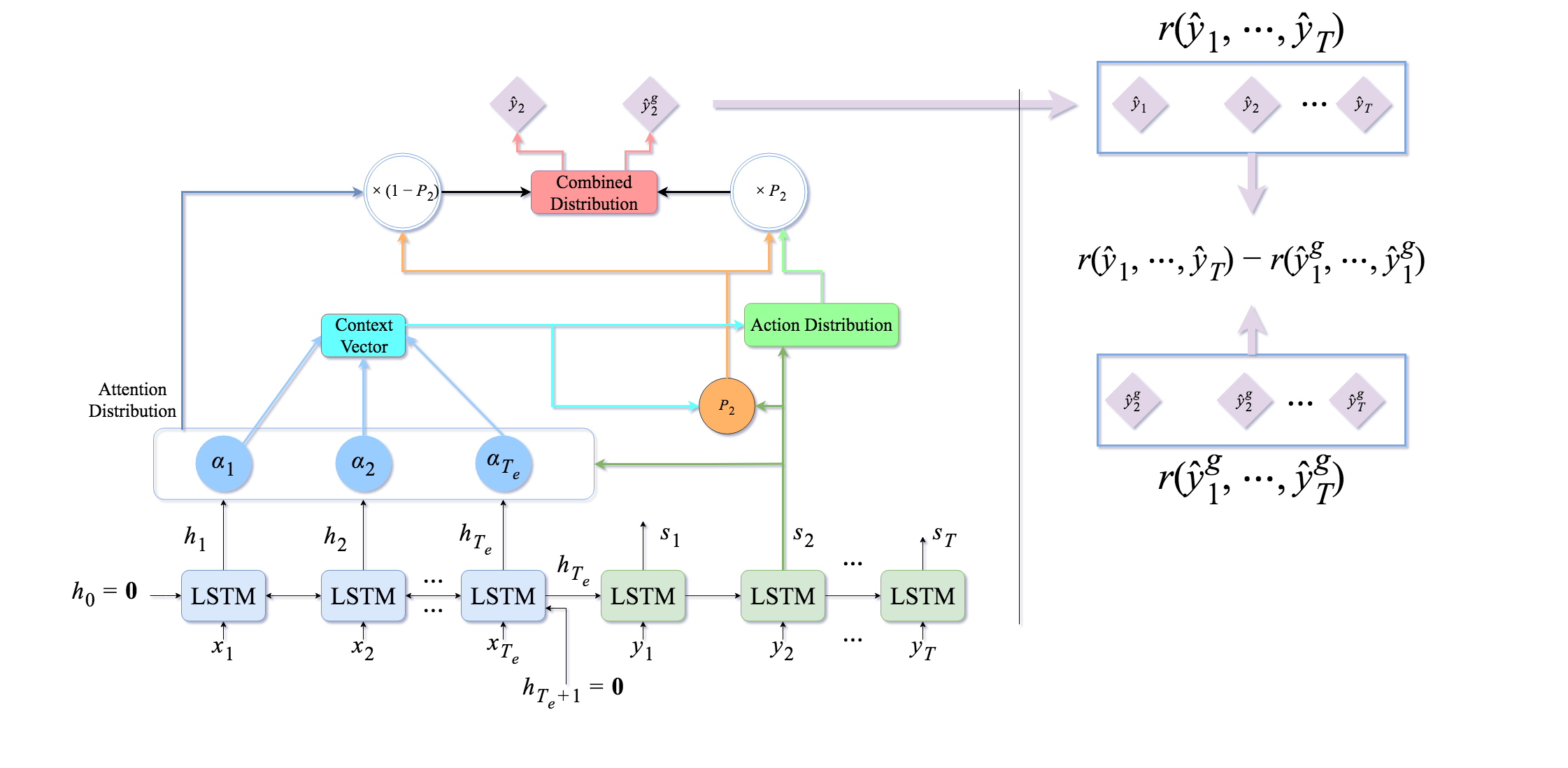
In recent years, different models and frameworks are suggested by researchers to achieve better and more robust results on these tasks. For instance, attention-based models has been successfully applied to problems such as machine translation [3], text summarization [9, 10], question answering [49], image captioning [19], speech recognition [16], and object detection [69]. In attention-based model, at each decoding time, we try to peak into the input and the encoder’s output to select the best decoder output. Fig. 2 shows an example of this model where the Action Distribution is generated from the attention distribution over the input and the current state of the decoder at time t=2. Although attention-based model will improve the performance of the seq2seq model significantly in different tasks, they have problems in applications where the output space is large. For instance, in the machine translation task, the decoder output is the word distribution over the vocabulary of the targeted language and size of this vector is equal to the number of words in that specific language (in order of millions). To avoid this huge vector size, we usually select only top-k words (like 50000 words) in our dataset. Therefore, it would be possible for the model to end up generating words that are not in the filtered vocabulary. These words are called Out of Vocabulary or OOV and we usually represent them with UNK symbol in our dataset. One of the problems, with attention-based model is that they are not offering any mechanism to handle these OOV outputs. Recently, pointer-generation models [70] are offered to solve this problem in text summarization. In these models, at each decoding step, we have a specific pointer that works like a switch. If this switch is on, we copy a word from the input and if the switch is off, we use the output of the model [71]. This way, if we have OOV in our output, we force the model to use the pointer and copy a word from the input. These models significantly reduce the number of OOVs in the final output and are shown to provide state-of-the-arts in text summarization tasks [12, 11]. There are more advanced models in seq2seq training like Transformers model which uses self-attention layers [72], but discussing these models is out of the scope of this paper.

2.1 Evaluation Metrics

Seq2seq model are usually trained with cross-entropy loss, i.e. Eq. (3). However, we evaluate the performance of these models with discrete measures. There are various discrete metrics that are used for evaluating these models and each application requires its own evaluation metric. We briefly provide a summary of these metrics according to their applications:

• ROUGE ⁴ [24], BLEU ⁵ [25], METEOR ⁶ [26]: These are three of the most common measure used in textual application such as machine translation, headline generation, text summarization, question answering, dialog generation, and any other application that requires evaluation over text data. ROUGE measure finds the common unigram (ROUGE-1), bigram (ROUGE-2), trigram (ROUGE-3), and largest common substring (LCS) (ROUGE-L) between a ground-truth text and the generated output by model and provides precision, recall, and F-score for these different measures. BLEU works similar to ROUGE but through a modified precision calculation, it suggests to provide higher scores to outputs that are closer to human judgement. In a similar approach, METEOR uses the harmonic mean of unigram precision and recall and it gives the recall higher scores than the precision. ROUGE and BLEU only focuses on word matching between the generated output and ground-truth document, but METEOR does the stemming and synonymy matching in addition to word matching. Although these methods are designed to work on all text applications, METEOR is used more often in machine translation tasks while ROUGE and BLEU are used mostly in text summarization, question answering, and dialog generation.

• CIDEr ⁷ [27], SPICE ⁸ [73]: CIDEr is frequently used in image and video captioning tasks in which having captions that have higher human judgement scores is more important. Using sentence similarity, the notions of grammaticality, saliency, importance, accuracy, precision, and recall are inherently captured by these metrics. To gain this, CIDEr first finds common n-grams between the generated output and the ground-truth and then calculates the TF-IDF value for them and takes the cosine similarity between the n-grams vectors. Finally, it combines a weighted sum of this cosine similarity for different values of n to get the evaluation measure.

  SPICE is a recent evaluation metric proposed for image captioning that tries to solve some of the problems of CIDEr and METEOR by mapping the dependency parse trees of the caption to the semantic scene graph (contains objects, attributes of objects, and relations) extracted from the image. Finally, it uses the F-score that is calculated using the tuples of the generated and ground-truth scene graphs to provide the caption quality score.

• Word Error Rate (WER): This measure which is mostly used in speech recognition, finds the number of substitutions, deletions, insertions, and corrections required to change the generated output to the ground-truth and combines them to calculate the WER. This is very much similar to the edit distance measures and this measure is sometimes considered as the normalized edit distance.

2.2 Datasets

In this section, we briefly talk about some of the common datasets that are used in different seq2seq models. In the past, researchers tested their models on various datasets and there was no standard and common dataset to evaluated different models and compare the performance of these models on a single unique dataset. However, recently with the help of open-source movement, the number of open datasets on different applications significantly increased. We provide a short list some of the most common datasets that are used in different seq2seq applications as follows:

• Machine Translation: The most common dataset in Machine Translation task is the WMT’14 ⁹ dataset which contains 850M words from English-French parallel corpora of UN (421M words), Europarl (61M words), news commentary (5.5M words), and two crawled corpora of 90M and 272.5M words. The data pre-processing on this dataset is usually done following Axelrod et al. [74] code ¹⁰.

• Text Summarization: One of the main dataset in text summarization is the CNN-Daily Mail dataset [75] which is part of the DeepMind Q&A Dataset ¹¹ and contains around 287K news articles along with 2 to 4 highlights (summary) for each news article ¹². This dataset was originally designed for question answering problem but later on used frequently for the text summarization. Along with our open-source library, we provide helper functions to clean and sentence-tokenize the articles in this dataset along with various metadata such as POS tagging and Named-Entities for the actual news article, highlights, and the title of the news. Our experiments show that using this cleaned version will provide much better results in the task of abstractive text summarization. Recently, another dataset called Newsroom is released by Connected Experiences Lab ¹³ [76] which contains 1.3M news articles and various metadata information such as the title and summary of the news. The document summarization challenge ¹⁴ also offers some datasets for text summarization. Most specifically in this dataset, DUC-2003 and DUC-2004 are used which contains 500 news article from the New York Times and Associated Press Wire services each paired with 4 different human-generated reference summaries, capped at 75 bytes. Due to the small size of this dataset, researchers usually use this dataset only for evaluations.

• Headline Generation: Headline generation is very similar to the text summarization and usually all the datasets that are used in text summarization will be useful in headline generation, too. Therefore, we can use CNN-Daily Mail, Newsroom, and DUC datasets for this purpose, too. However, there is another big dataset which is called Gigaword [77] and contains more than 8M news articles from multiple news agencies like New York Times, Associate Press, Agence France Press, and The Xinhua News Agency. However, this dataset is not free and researchers are required to buy the license to be able to use this dataset but we can still find pre-trained models on different tasks using this dataset ¹⁵.

• Question Answering, Question Generation: As mentioned above, CNN-Daily Mail dataset was originally designed for question answering and is one of the earliest dataset for this problem. However, recently two big datasets are released which are solely designed for this problem. Stanford Question Answering Dataset (SQuAD) ¹⁶ [78] is a dataset for reading comprehension and contains more than 100K pairs of questions and answers collected by crowdsourcing over a set of Wikipedia articles. The answer to each question is a segment where identifies the start and end index of the answer in the article. The second dataset is called TriviaQA ¹⁷ [79] and similar to SQuAD is designed for reading comprehension and question answering task. This dataset contains, 650K triples of questions, answers, and evidences (which helps to find the answer). The SimpleQuestions dataset [80] is another dataset that contains more than 108K questions written by English-speaking human. Each question is paired with a corresponding fact, formatted as triplet (subject, relationship, object), that provides the answer along with a thorough explanation. WikiQA [81] dataset offers another challenging dataset which contains pairs of question and answers collected from Bing queries. Each question is then linked to a Wikipedia page that potentially has the answer and consider the summary section of each wiki page as the answer sentences.

• Dialogue Generation: The dataset for this problem usually comprises of dialogues between different people. The OpenSubtitles dataset ¹⁸ [82], Movie Dialog dataset ¹⁹ [83], and Cornell Movie Dialogs Corpus ²⁰ [84] are three examples of these types of datasets. OpenSubtitles contains conversations between movie characters for more than 20K movies in 20 languages. The Cornell Movie Dialogs contains more than 220K dialogs between more than 10K movie characters. Some researchers used conversations in an IT desk [51] while others used Twitter to extract conversations among different users [52, 85]. However, none of these two datasets are open-sourced.

• Image Captioning: There are three datasets that are mainly used in image captioning. The first one is the COCO dataset ²¹ [86] which is designed for object detection, segmentation, and image captioning. This dataset contains around 330K images which among them there are 82K images used for training and 40K used for validation in image captioning. Each image has five ground-truth captions. SBU [87] is another dataset which consists of 1M images from Flickr and contains descriptions provided by image owners when they uploaded them to Flickr. Lastly, the Pascal dataset [88] is a small dataset containing 1000 image-caption pairs which only used for testing purposes.

• Video Captioning: In this problem, MSR-VTT ²² [89] and YouTube2Text/MSVD ²³ [90] are two of the frequently used datasets where MSR-VTT contains 10K videos from a commercial video search engine each containing 20 human annotated captions and YouTube2Text/MSVD which has 1970 videos each containing on average 40 human annotated captions.

• Computer Vision: The most famous dataset in computer vision is MNIST dataset ²⁴ [91]. This dataset contains handwritten digits and contains a training set of 60K examples and a test set of 10K examples. Aside from this dataset, there is a huge list of datasets that are used in various computer vision problems and explaining each of them is beyond the scope of this paper ²⁵.

• Speech Recognition: LibriSpeech ASR Corpus ²⁶ [92] is one of the main datasets for speech recognition task. This dataset is free and composed of 1000 hours of segmented and aligned 16kHz English speech which is derived from audiobooks. Wall Street Journal (WSJ) also has two Continuous Speech Recognition (CSR) corpora containing 70 hours of read speech and text from a corpus of Wall Street Journal news text. However, unlike the LibriSpeech dataset, this dataset is not free and researcher has to buy a license to use it. Similar to the WSJ dataset, TIMIT ²⁷ is another dataset containing the read speech data. It contains time-aligned orthographic, phonetic, and word transcriptions of recordings for 630 speakers of eight major dialects of American English in which each reading ten phonetically sentences.

3 Methods of Reinforcement Learning

In reinforcement learning, the goal of an agent interacting with an environment is to maximize the expectation of the reward that it receives from the actions. Therefore, we are trying to maximize one of these objectives:

Maximize E^y1,⋯,^yT∼πθ(^y1,⋯,^yT)[r(^y1,⋯,^yT)]

(9)

Maximizey Aπ(st,yt)

(10)

Maximizey Aπ(st,yt)→Maximizey Qπ(st,yt)

(11)

There are various ways, we can solve this problem. In this section, we explain each of these solutions in details and provide their strength and weaknesses. Some methods try to solve this problem through Eq. (9), some try to solve the expected discounted reward E[Rt=∑Tτ=tγτ−trτ], some try to solve it by maximizing the advantage function (Eq. (10)), and last but not least we can solve this problem by maximizing Q function using Eq. (11). Most of these methods are suitable choice for improving seq2seq models, but depending on which model we choose to train the reinforced model, the training process for seq2seq model also changes. The first and easiest algorithm that we discuss in this section is the Policy Gradient (PG) method which aims to solve Eq. (9). Section 3.2 discusses Actor-Critic (AC) models which improve the PG models by solving Eq. (10) through Eq. (7) extension. Section 3.3 talks about Q-learning models that use maximization over the Q function (Eq. (11)) to improve the PG and AC models. Finally, Section 3.4 talks about some of the recents models which improve Q-learning models.

3.1 Policy Gradient

In all reinforcement algorithm, an agent takes some action according to a specific policy π. The definition of policy in different application is different. For instance, in text summarization, the policy is a language model p(y|X) that given input X tries to generate the output y. Let’s assume that our agent is represented by an RNN and takes actions from a policy πθ²⁸. In a deterministic environment, where agent takes discrete actions, the output layer of the RNN is usually a softmax function and it generates output from this layer. In Teacher Forcing, we have a set of ground-truth sequences and during training we choose actions according to the current policy and only observe a reward at the end of the sequence or when we see an End-Of-Sequence (EOS) signal. Once the agent reaches the end of sequence, it compares the sequence of actions from the current policy (^yt) against the ground-truth action sequence (yt) and calculate a reward based on the evaluation metric. The goal of training is to find the parameters of the agent in order to maximize the expected reward. We define this loss as the negative expected reward of the full sequence:

Lθ=−E^y1,⋯,^yT∼πθ(^y1,⋯,^yT)[r(^y1,⋯,^yT)]

(12)

where ^yt is the action chosen by model at time t and r(^y1,⋯,^yT) is the reward associated with the actions ^y1,⋯,^yT. Usually in practice, we approximate this expectation with a single sample from the distribution of actions implemented by the RNN. Therefore, the derivative for the above loss is as follows:

∇θLθ=−E^y1⋯T∼πθ[∇θlogπθ(^y1⋯T)r(^y1⋯T)]

(13)

Using the chain rule, we can write down this equation as follows [93]:

∇θLθ=∂Lθ∂θ=∑t∂Lθ∂ot∂ot∂θ

(14)

where ot is the input to the softmax function. The gradient of the loss Lθ with respect to ot is given by [93, 94]:

∂Lθ∂ot=(πθ(yt|^yt−1,st,ct−1)−1(^yt))(r(^y1,⋯,^yT)−rb)

(15)

where 1(^yt) is the 1-of-|A| representation of the ground-truth output and rb is a baseline reward and could be any value as long as it is not dependent on the parameter of the RNN network. This equation is quite similar to the gradient of a multi-class logistic regression. In logistic regression, the cross-entropy gradient is the difference between the prediction and the actual 1-of-|A| representation of the ground-truth output:

∂LCEθ∂ot=πθ(yt|yt−1,st,ct−1)−1(yt)

(16)

Note that in Eq. (15), we use the generated output from the model as the surrogate ground-truth for the output distribution while in Eq. (16) we use the ground-truth to calculate the gradient.

The goal of the baseline reward is to force the model to select actions that yield a reward r>rb and discourage those that have reward r<rb. Since we are using only one sample to calculate the gradient of loss, it is shown that having this baseline would reduce the variance of the gradient estimator [94]. If the baseline is not dependent on the parameters of the model θ, Eq. (15) is an unbiased estimator. To prove this, we simply need to show that adding the baseline reward rb does not have any effect on the expectation of loss:

E^y1⋯T∼πθ[∇θlogπθ(^y1⋯T)rb]=rb∑^y1⋯T∇θπθ(^y1⋯T)=rb∇θ∑^y1⋯Tπθ(^y1⋯T)=rb∇θ1=0

(17)

This algorithm is called REINFORCE [94] and is a simple yet elegant policy gradient algorithm for seq2seq problems. One of the problems with this method is the use of only one sample to train the model at each time step, therefore the model suffers from high variance. To alleviate this problem, at each training step we can sample N sequences of actions and update the gradient by averaging over all these N sequences:

Lθ=1N∑Ni=1∑tlogπθ(yi,t|^yi,t−1,si,t,ci,t−1)×(r(^yi,1,⋯,^yi,T)−rb)

(18)

Having this, we can set the baseline reward to be the mean of the N rewards that we sampled, i.e. rb=1/N∑Ni=1r(^yi,1,⋯,^yi,T). Algorithm 2 shows how this method works.

As another solution to reduce the variance of the model, Self-Critic (SC) models are proposed where rather than estimating the baseline using current samples, we use the output of the model obtained by a greedy-search (the output at the time of inference) as the baseline. Therefore, we use the sampled output of the model as ^yt and use greedy selection of the final output distribution for ^ygt where superscript g means greedy selection. This way the new objective for the REINFORCE model would be as follows:

Lθ=1N∑Ni=1∑tlogπθ(yi,t|^yi,t−1,si,t,ci,t−1)×(r(^yi,1,⋯,^yi,T)−r(^ygi,1,⋯,^ygi,T))

(19)

Fig 2 shows how we can use an attention-based pointer-generator seq2seq model to extract the reward and its baseline in Self-Critic model.

Input: Input sequences, X, ground-truth output sequences, Y, and preferably a pre-trained policy, πθ. Output: Trained policy with REINFORCE. Training Steps: while not converged do       Select a batch of size N input and output sequences, X and Y.       Sample N full sequence of actions:       {^y1,⋯,^yT∼πθ(^y1,⋯,^yT)}N1.       Observe the sequence reward and calculate the baseline rb.       Calculate the loss according to Eq. (18).       Update the parameters of network θ←θ+α∇θLθ. end while Testing Steps: for batch of input and output sequences X and Y do       Use the trained model and Eq. (4) to sample the output ^Y.       Evaluate the model using a performance metric, e.g. ROUGEl. end for

The second problem with this method is that we only observe the reward after the full sequence of actions is sampled. This might not be a pleasing feature for most of the seq2seq models. If we see the partial reward of a given action at time t, and the reward is bad, the model needs to select a better action for the future to maximize the reward. However, in the REINFORCE algorithm, the model is forced to wait till the end of the sequence to observe its performance. Therefore, the model often generates poor results or takes longer to converge. This problem magnifies especially in the beginning of the training phase where the model is initialized randomly and thus selects arbitrary actions. To somehow alleviate this problem, Ranzato et al. [28] suggested to pre-train the model for a few epochs using the cross-entropy loss and then slowly switch to the REINFORCE loss. Finally, as another way to solve the high variance problem of REINFORCE algorithm we can use importance sampling [95, 96]. The underlying idea in using importance sampling with REINFORCE algorithm is that rather than sampling sequences from the current model, we sample them from an old model and use them to calculate the loss.

3.2 Actor-Critic Model

As mentioned in Section 3.1, adding a baseline reward is a necessary part of the PG algorithm to reduce the variance of the model. In PG, we used the average reward from multiple samples in the batch as the baseline reward for our model. In Actor-Critic (AC) model, we try to train an estimator to calculate the baseline reward. To do this, AC models try to maximize the advantage function through Eq. (7) extension. Therefore, these methods are also called Advantage Actor-Critic (AAC) models.

We are trying to solve this problem with the following objective:

Aπ(st,yt)=Qπ(st,yt)−Vπ(st)=rt+γEst′∼π(st′|st)[Vπ(st′)]−Vπ(st)

(20)

Similar to PG algorithm to avoid the expensive inner expectation calculation, we can only sample once and approximate advantage function as follows:

Aπ(st,yt)≈rt+γVπ(st′)−Vπ(st)

(21)

Now, in order to estimate Vπ(s), we can use a function approximator to approximate the value function. In AC, we usually use neural networks as the function approximator for the value function. Therefore, we fit a neural network Vπ(s;Ψ) with parameters Ψ to approximate the value function. Now, if we think of rt+γVπ(st′) as the expectation of reward-to-go at time t, Vπ(st) could play as a surrogate for the baseline reward. Similar to the PG, since we are only using one sample to train the model the variance would be high. Therefore, we can reduce the variance again using multiple samples. In AC model, the Actor (our policy, θ) provides samples (policy states at time t and t+1) for the Critic (neural network estimating value function, Vπ(s;Ψ) and Critic returns the estimation to the Actor and finally Actor uses these estimations to calculate the advantage approximation and update the loss according to the following equation:

Lθ=1N∑Ni=1∑tlogπθ(yi,|^yi,t−1,si,t,ci,t−1)AΨ(si,t,yi,t)

(22)

Therefore, in the AC models, the inference at each time t would be as follows:

argmaxyπθ(yt|^yt−1,st,ct−1)AΨ(st,yt)

(23)

Fig. 3 shows this model.

Training Critic Model

As mentioned in the previous section, the Critic is a function estimator which tries to estimate the expected reward-to-go for the model at time t. Therefore, training the Critic is basically a regression problem. Usually, in AC models, we use a neural network as the function approximator and we train the value function using the mean square error:

L(Ψ)=12∑i||VΨ(si)−vi||2

(24)

where vi=∑Tt′=tr(si,t′,yi,t′) is the true reward-to-go at time t. During training the Actor model, we collect (si,vi) pairs and pass them to the Critic model to train the estimator. This model is called on-policy AC meaning that we rely on the samples that are collected at the current time to train the Critic model. However, the samples that are passed to Critic will be correlated to each other and causes poor generalization for the estimator. We can make these methods off-policy by collecting training samples into a memory buffer and select mini-batches from this memory buffer and train the Critic network. Off-policy AC provides a better training due to avoiding the correlation of samples that exists in the on-policy methods. Therefore, most the models that we talk about in this paper are mostly off-policy and use a memory buffer for training the Critic model.

Algorithm 3 shows the training process of AAC model. Algorithm 3 shows the batch AAC algorithm since for training the Critic network, we use a batch of state-rewards pair. In the online AAC algorithm, we simply update the Critic network using just one sample and as expected online AAC algorithm has a higher variance due to the fact that we only use one sample to train the network. To alleviate this problem for online AAC, we can use Synchronized AAC (SAAC) learning or Asynchronized AAC (A3C) learning [97]. In SAAC, we use N different threads to train the model and each thread does the online AAC for one sample and at the end of the algorithm, we use the gradient of these N threads to update the gradient of the Actor model. In the more common A3C algorithm, as soon as a thread calculates θ, it will send the update to other threads and other threads use the new updated θ to train the model. A3C is an on-policy method with multi-step returns while there are other methods like Retrace [98], UNREAL [99], and Reactor [100] which provide the off-policy variations of this model by using the memory buffer. Also, ACER [101] mixes on-policy (from current run) and off-policy (from memory) to train the Critic network.

Input: Input sequences, X, ground-truth output sequences, Y, and preferably a pre-trained Actor model, πθ. Output: Trained Actor and Critic models. Training Steps: Initialize the Actor (Seq2seq) model, πθ. Initialize the Critic (ValueNet) model, VΨ. while not converged do       Training Actor:       Select a batch of size N input and output sequences X and Y.       Sample N full sequences of actions based on the Actor.       model, πθ.       for n=1,⋯,N do             for t=1,⋯,T do                  Calculate the true (discounted) reward-to-go:                  vt=∑Tt′=tγt′−tr(si,t′,yi,t′).                  Store training pairs for Critic: (st,vt).             end for       end for              Training Critic:       Select a batch of size Nc from the pool of state-rewards pairs.       collected from Actor.       for n=1,⋯,Nc do             Collect the value estimates ^vn from VΨ for each             state-rewards pair.       end for       Minimize the Critic loss using Eq. (24).              Updating Actor:       Use the estimated value for VΨ(st) and VΨ(st′)       to calculate the loss using Eq. (22).       Update parameters of the model using θ←θ+α∇θL(θ). end while

In general, AC models usually have low variance due to the batch training and use of critic as the baseline reward, but they are not unbiased if the critic is not perfect and makes a lot of mistakes. As mentioned in Section 3.1, PG algorithm has high variance but it provides an unbiased estimator. Now, if we combine the PG and AC model, we are likely end up with a model that has no bias and low variance. This idea comes from the fact that for deterministic policies (like seq2seq models), we can derive a partially observable loss using the Q-function as follows [102, 103]:

Lθ=1N∑Ni=1∑tlogπθ(yi,t|^yi,t−1,si,t,ci,t−1)×(QΨ(si,t)−VΨ′(si,t))

(25)

However, this model requires training two different models for QΨ function and VΨ′ function as the baseline. Note that we cannot use the same model to estimate both Q function and value function since the estimator will not be an unbiased estimator anymore [104]. As yet another solution to create a trade-off between the bias and variance in AC, Schulman et al. [105] proposed the Generalized Advantage Estimation (GAE) model as follows:

AGAEΨ(st,yt)=T∑i=t(γλ)i−t(r(si,yi)+γVΨ(si+1)−VΨ(si))

(26)

where λ controls the trade-off between the bias and variance such that big values of λ yield to larger variance and lower bias, while small values of λ do the opposite.

3.3 Actor-Critic with Q-Learning

As mentioned in previous section, we used the value function to maximize the advantage function. As an alternative to solve the maximization of advantage estimates, we can try to solve the following objective function:

Maximizey Aπ(st,yt)→Maximizey Qπ(st,yt)−Vπ(st)0

(27)

This is true since we are trying to find the actions that maximize the advantage estimate and since value function does not rely on the actions, we can simply remove them from the maximization objective. Therefore, we simplified the advantage maximization problem to Q function estimation problem. This method is called Q-learning and it is one of the most common algorithm used in RL. In Q-learning, the Critic tries to provide estimation for the Q-function. Therefore, given that you are using the policy πθ, our goal is to maximize the following loss at each training step:

Lθ=1N∑Ni=1∑tlogπθ(yi,t|^yi,t−1,si,t,ci,t−1)QΨ(si,t,yi,t)

(28)

Similar to the value network training, the Q-function estimation is a regression problem and we need to use the Mean Squared Error to estimate these values. However, one of the differences between the Q-function training and value function training is the way we choose our true estimates. In value function estimation, we use the ground-truth data to calculate the true reward-to-go as vi=∑Tt′=tr(si,t′,yi,t′), however in Q-learning we use the estimation from the network approximator itself to train the regression model:

(29)

where s′i and y′i are the state and action at the next time, respectively. Although our Q-value estimation has no direct relation to the true Q-values calculated using ground-truth data, in practice it is known to provide good estimation and provides a much faster training due to not collecting ground-truth reward at each step of the training. However, there are no rigorous study on really how far are these estimates from the true Q-values. As you can see in Eq. (29), the true Q estimations is calculated using the estimation from network approximator at time t+1, i.e. max′yQΨ(s′i,y′i). Although, not relying on the true ground-truth estimation and explicitly using the reward function might seems to be a bad idea, however in practice it is shown that these models provide better and more robust estimators. Therefore, the training process in Q-learning consists of first collecting a dataset of experiences et=(st,yt,st′,rt) during training our Actor model and then use them to train the network approximator. This is the standard way of training the Q-network and was frequently used in earlier temporal-difference learning models. But, there is a problem with this method. Generally, the Actor-Critic models with neural network as function estimator are tricky to train and unless we make sure that the estimator is good, the model will not converge. Although the original Q-learning method is proved to converge [106, 107], when we use neural networks to approximate the estimator, the convergence guarantee will vanish. Usually, since samples are coming from a specific sets of sequences, there is a correlation between the samples that we choose to train the model. Thus, this may cause any small updates to Q-network to significantly change the data distribution, and ultimately affects the correlations between Q and the target values. Recently, Mnih et al. [35] proposed the idea of using an experience buffer²⁹ to store the experiences from different sequences and then randomly select a batch from this dataset and train the Q-network. Similar to the off-policy AC model, one benefit of using this buffer is to increase efficiency of the model by re-using the experiences in multiple updates and reducing the variance of the model. Since by sampling uniformly from the buffer, we reduce the correlation of samples used in the updates. As another improvement to the experience buffer, we can use a prioritized version of this buffer in which, to select our mini-batches during training, we only select samples that have higher rewards [108]. Algorithm 4 provides the pseudo-code for a Q-learning algorithm called Deep Q-Network or DQN.

Input: Input sequences, X, ground-truth output sequences, Y, and preferably a pre-trained Actor model, πθ. Output: Trained Actor and Critic models. Training Steps: Initialize the Actor (Seq2seq) model, πθ. Initialize the Critic (Q-Net) model, QΨ. while not converged do       Training Seq2seq Model:       Select a batch of size N input and output sequences X and Y.       Sample N full sequences of actions based on the Actor       model, πθ.       for n=1,⋯,N do             for t=1,⋯,T do                  Collect experience et=(st,yt,st′,rt) and                  add them to the experience buffer.             end for       end for              Training Q-Net:       Select a batch of size Nq from the experience buffer.       based on the reward.       for n=1,⋯,Nq do             Estimate ^qn=QΨ(sn,yn).             Calculate the true estimation:                          Store (^qn,qn).       end for       Updating Q-Net:       Minimize the loss using Eq. (29).       Update the parameters of network, Ψ.              Updating Seq2seq Model:       Use the estimated Q values for ^qn=QΨ(sn,yn).       to calculate the loss using Eq. (28).       Update parameters of the model using θ←θ+α∇θL(θ). end while

3.4 Advanced Q-Learning

Double Q-Learning

One of the problems with the Deep Q-Network (DQN) is the overestimation of Q-values as shown in [109, 110]. Specifically, the problem lies in the fact that we do not use the ground-truth reward to train these models and use the same network to calculate both the estimation of network QΨ(si,yi) and true values for regression training, qi. To alleviate this problem, we can use two different networks in which one chooses the best action when calculating maxy′QΨ(s′n,y′n) and the other calculate the estimation of Q value, QΨ(si,yi). In practice, we use a modified version of the current DQN network as the second network in which we freeze the current network parameters for a certain period of time and update the second network, periodically. Let’s call the second network our target network with parameters Ψ′. We know that maxy′QΨ(s′n,y′n) is the same as choosing the best action according to the network QΨ. Therefore, we can re-write this equation as QΨ(s′t,argmaxy′tQΨ(s′t,y′t)). As you can see in this equation, we use QΨ for both calculating the Q-value and finding the best action. Given that we have a target network, we can choose the best action using our target network and do the estimation using our current network. Therefore, using the target network, QΨ′ the Q-estimation will be as follows:

(30)

where EOS is the End-Of-Sequence action. This method is called Double DQN [109, 111] and is shown to resolve the problem of overestimation in DQN and provides more realistic estimations. But, even this model suffers from the fact that there is no relation between the true Q-values and the estimation provided by the network. Algorithm 5 shows the pseudo-code for this model.

Input: Input sequences, X, ground-truth output sequences, Y, and preferably a pre-trained Actor model, πθ. Output: Trained Actor and Critic models. Training Steps: Initialize the Actor (Seq2seq) model, πθ. Initialize the two Critic models: current Q-Net, QΨ, and target Q-net, QΨ′: QΨ′←QΨ. while not converged do       Training Seq2seq Model:       Select a batch of size N input and output sequences X and Y.       Sample N full sequences of actions based on the Actor       model, πθ.       for n=1,⋯,N do             for t=1,⋯,T do                  Collect experience et=(st,yt,st′,rt) and                  add them to the experience buffer.             end for       end for              Training Q-Net:       Select a batch of size Nq from the experience buffer       based on the reward.       for n=1,⋯,Nq do             Estimate ^qn=QΨ(sn,yn)             Calculate the true estimation:                          Store (^qn,qn).       end for       Updating current Q-Net:       Minimize the loss using Eq. (29).       Update the parameters of network, Ψ.              Updating target Q-Net every Nu iterations:       Ψ′←Ψ or using Polyak averaging:       Ψ′←τΨ′+(1−τ)Ψ, τ=1000−(Current Step%1000)1000.              Updating Seq2seq Model:       Use the estimated Q-values for ^qn=QΨ(sn,yn)       to calculate the loss using Eq. (28).       Update parameters of the model using θ←θ+α∇θL(θ). end while

Dueling Networks

In DDQN, we tried to solve one of the problems with DQN model by using two networks in which the target network selects the next best action while the current network estimates the Q-values given the action selected by target. However, in most applications it is unnecessary to estimate the value of each action choice. This is specially of importance for discrete problems with a large sets of possible actions where only a few actions are actually good. For instance, in text summarization the output of the model is a vector of the distribution over the vocabulary and therefore, the output has the same dimension as the vocabulary size which is usually selected to be between 50K to 150K. In most of the applications that uses DDQN, the action space is limited to less than a few hundred. For instance, in an Atari game, the possible actions could be to move left, right, up, down, and shoot. Therefore, using DDQN would be easy for these types of application. Recently, Wang et al. [112] proposed the idea of using a dueling net to overcome this problem. In their proposed method, rather estimating the Q-values directly from the Q-net, we try to estimate two different values for the value function and advantage function as follows:

QΨ(st,yt)=VΨ(st)+AΨ(st,yt)

(31)

In order to be able to calculate the VΨ(st), we need to replicate the value estimates, |A| times. However, as discussed in [112], using Eq. (33) to calculate the Q is a bad idea and cause poor performance since Eq. (33) is unidentifiable in the sense that we can simply add a constant to VΨ(st) and subtract the same constant from AΨ(st,yt). To solve this problem, the author suggested to force the advantage estimator to have a zero at the selected action:

QΨ(st,yt)=VΨ(st)+(AΨ(st,yt)−maxyAΨ(st,y))

(32)

This way for the action y∗=argmaxyQΨ(st,y)=argmaxyAΨ(st,y), we obtain QΨ(st,y∗)=VΨ(st). As an alternative to Eq. (32) and to make the model more stable, the author suggested to replace the max operator with average:

QΨ(st,yt)=VΨ(st)+(AΨ(st,yt)−1|A|∑yAΨ(st,y))

(33)

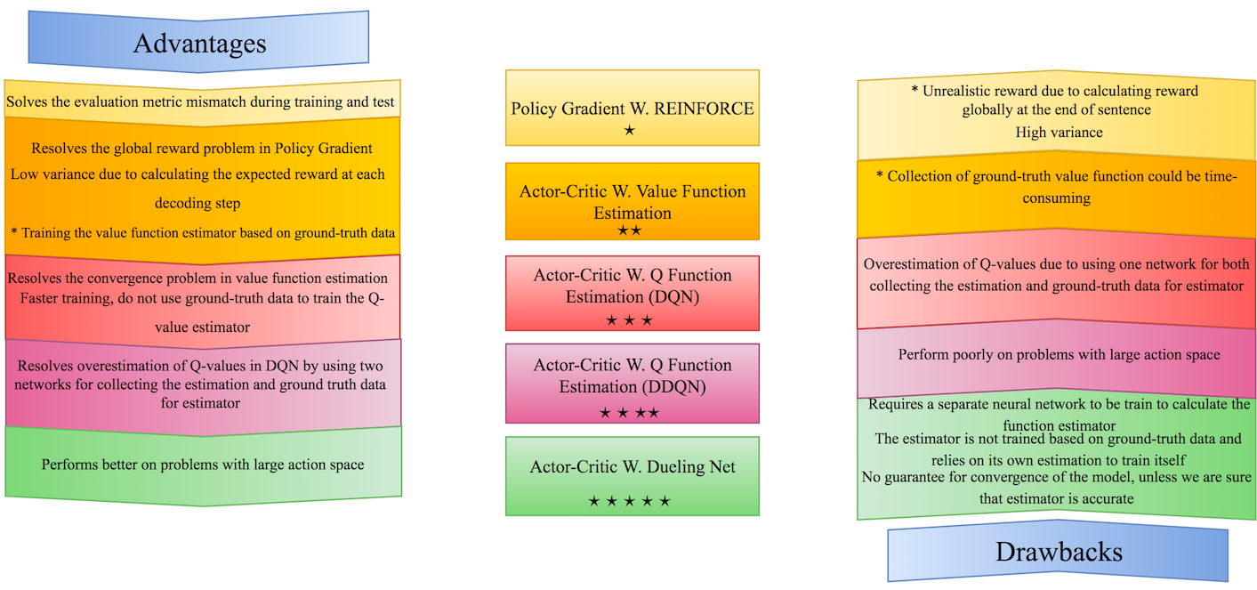
Similar to DQN and DDQN, this model also suffers from the fact that there is no relation between the true values of Q-function and the estimation provided by the network. In Section 5, we propose a simple and effective solution to overcome this problem by doing schedule sampling between the Q-value estimations and true Q-values to pre-train our function approximator. Fig. 4 summarizes some of the strengths and weaknesses of these different RL methods.

4 Combining RL with Seq2seq Models

In this section, we will provide some of the recent models that combined the seq2seq training with Reinforcement Learning. In most of these models, the main goal is to solve the train/test evaluation mismatch problem, that exists in all previous models, by adding a reward function to the training model. There are a growing number of researchs that used the REINFORCE algorithm to improve the current state-of-the-art seq2seq models. However, more advanced techniques such as Actor-Critic models, DQN, and DDQN has not been used that often for these tasks. As mentioned before, one the main difficulties of using Q-Learning and its derivatives, is the large action space for seq2seq models. For instance, in a text summarization task, the model should provide estimates for each word in the vocabulary and therefore the estimation could be really poor even with a good trained model. Due to these reasons, researchers mostly focused on the easier yet problematic approaches such as REINFORCE algorithm to train the seq2seq model. Therefore, combining the power of Q-Learning training to seq2seq model is still considered an open area for the researchers. Table IV summarizes these models along with the respective seq2seq application and RL model they used to improve that application. Moreover, Table III explains what are the policy, action, and reward function for each seq2seq task.

Seq2seq Task	Policy	Action	Reward
Text Summarization Headline Generation Machine Translation Question Generation	Attention-based models, pointer-generators, etc	Selecting the next token for summary, headline, and translation	ROUGE, BLEU
Question Answering	Seq2seq model	Selecting the answer from a vocabulary or selecting the start and end index of the answer in the input document	F1 Score
ImageCaptioning Video Captioning	seq2seq model	Selecting the next token for the caption	CIDEr, SPICE, METEOR
Speech Recognition	Seq2seq model	Selecting the next token for the speech	Connectionist Temporal Classification (CTC)
Dialog Generation	Seq2seq model	Dialogue utterance to generate	BLEU Length of dialogue Diversity of dialogue

4.1 Policy Gradient and REINFORCE Algorithm

As mentioned in Section 3.1, in Policy Gradient (PG), we observe the reward of the sampled sequence at the end of the sequence generation and back-propagate that error equally to all the decoding steps according to Eq. (15). Also, we talked about the exposure bias problem that exists in seq2seq models during training the decoder because of using Cross-Entropy (CE) error. The idea of improving generation by letting the model use its own predictions at training time was first proposed by Daume III et al. [113]. Based on their proposed method, SEARN, the structured prediction problems can be cast as a particular instance of reinforcement learning. The basic idea is to let the model use its own predictions at training time to produce a sequence of actions (e.g., the choice of the next word). Then, a greedy search algorithm is run to determine the optimal action at each time step, and the policy is trained to predict that action. An imitation learning framework was proposed by Ross et al. [114] in a method called DAGGER, where an oracle of the target word given the current predicted word is required. However, for tasks such as text summarization, computing the oracle is infeasible due to the large action space. This problem later on addressed by the Data As Demonstrator (DAD) model [115], where the target action at step k is the kth action taken by the optimal policy. One drawback of DAD is that at every time step the target label is always selected from the ground-truth data and if the generated summaries are shorter than the ground-truth summaries, the model still forces to generate outputs that could already exist in the model. One way to avoid this problem in DAD is to use a method called End2EndBackProp [28] in which at each step t, we get the top-k actions from the model and use the normalized probabilities of these actions to weight their importance and feed the normalized combination of their representation to the next decoding step.

Finally, REINFORCE algorithm [94] tries to overcome all these problems by using the PG rewarding function and avoiding the CE loss by using the sampled sequence as the ground-truth to train the seq2seq model, Eq. (18). In real-world applications, we usually start the training with the CE loss and acquire a pre-trained model. Then, we move on to use the REINFORCE algorithm to train the model. As some of the earliest adoptions of REINFORCE algorithm for training seq2seq models are in computer vision [116, 69], image captioning [19], and speech recognition [67]. Recently, other researchers showed that using a combination of CE loss and REINFOCE loss could yield a better result than just simply doing the pre-training. In these models, we start the training using the CE loss and slowly switch from CE loss to REINFORCE loss to train the model. There are various way, we can do the transition from CE loss to REINFORCE loss. Ranzato et al. [28] used an incremental scheduling algorithm called MIXER in which combines the DAGGER [114] and DAD [115] methods. In this method, we train the RNN with the cross-entropy loss for NCE epochs using the ground-truth sequences. This ensures that the model starts off with a much better policy than random because now the model can focus on the good part of the search space. Then, they use an annealing schedule in order to gradually teach the model to produce stable sequences. Therefore, after the initial NCE epochs, they continue training the model for NCE+NR epochs, such that, for every sequence they use the LCE for the first (T−δ) steps, and the REINFORCE algorithm for the remaining δ steps. The MIXER model was successfully used on a variety of tasks such as text summarization, image captioning, and machine translation.

Another way to handle the transition from using CE loss to REINFORCE loss is to use the following combined loss:

Lmixed=ηLREINFORCE+(1−η)LCE

(34)

where η∈(0,1) is the parameter that controls the transition from CE to REINFORCE loss. In the beginning of the training η=0 and the model completely relies on CE loss, while as we move on with the training we can increase the η to slowly reduce the effect of CE loss. By the end of the training process where η=1, we are completely using the REINFORCE loss to train the model. This mixed training loss has been used in many of the recent works on text summarization [13, 36, 117], image captioning [?], video captioning [118], speech recognition [119], dialogue generation [120], question answering [121], and question generation [47].

4.2 Actor-Critic Models

One of the problems with the PG model is that we need to sample the full sequences of actions and observe the reward at the end of generation. This in general will be problematic since the error of generation accumulates over time and usually for long sequences of actions, the final sequence is so far away from the ground-truth sequence. Thus, the reward of the final sequence would be small and model would take a lot of time to converge. To avoid this problem, Actor-Critic models observe the reward at each decoding step using the Critic model and fix the sequence of future actions that the Actor is taking. The Critic model usually tries to maximize the advantage function through estimation of value function or Q-function. As one of the early attempts of using AC models, Bahdanau et al. [102] and He et al. [122] used this model on machine translation. In [102] the author used temporal-difference (TD) learning for advantage function estimation through estimation of Q-value for the next action, i.e. Q(st,yt+1), as a surrogate for the true estimate for the value estimation at time t, i.e. VΨ(st). We mentioned that for a deterministic policy, y∗=argmaxyQ(s,y), it follows that Q(s,y∗)=V(s). Therefore, we can use the Q-value for the next action as the true estimates of the value function at current time. To accommodate for the large action space, they also use the shrinking estimation trick that was used in dueling net to push the estimate to be close their means. Additionally, the Critic training is done through the following mixed objective function:

L(Ψ)=12∑i||QΨ(si,yi)−qi||2+η¯Qi¯Qi=∑y(QΨ(y,si)−1|A|∑y′QΨ(y′,si))

(35)

where qi is the true estimation of Q from a delayed Actor. The idea of using delayed Actor is similar to the idea used in Double Q-Learning where we use a delayed target network to get estimation of the best action. Later on Zhang et al. [123] used a similar model on image captioning task.

He et al. [122], proposed a value network that uses a semantic matching and a context-coverage module and passed them through a dense layer to estimate the value function. However, their model requires a fully-trained seq2seq model to train the value network. Once the value network is trained, they use the trained seq2seq model and trained value estimation model to do the beam search during translation. Therefore, the value network is not used during the training of the seq2seq model. During inference, however, similar to the AlphaGo model [34], rather multiplying the advantage estimates (or value or Q estimates) to the policy probabilities like in Eq. (23), they combine the output of the seq2seq model and the value network as follows:

η×1Tlogπ(^y1⋯T|X)+(1−η)×logVΨ(^y1⋯T)

(36)

where VΨ(^y1⋯T) is the output of the value network and η controls the effect of each score.

In a different model, Li et al. [124] proposed a model that controls the length of seq2seq model using ideas from RL. They train a Q-value function approximator which estimates the future outcome of taking an action yt in the present and then incorporate it into a score S(yt) at each decoding step as follows:

S(yt)=logπ(yt|yt−1,st)+ηQ(X,y1⋯t)

(37)

Specifically, the Q function, in this work, takes only the hidden state at time t and estimates the length of the remaining sequence. While decoding, they suggest an inference method that controls the length of the generated sequence as follows:

^yt=argmaxylogπ(y|^y1⋯t−1,X)−η||(T−t)−QΨ(st)||2

(38)

Recently, Li et al. [36] proposed an AC model which uses a binary classifier as the Critic. In this specific model, the Critic tries to distinguish between the generated summary and the human-written summary via a neural network binary classifier. Once they pre-trained the Actor using CE loss, they start training the AC model alternatively using PG and the classifier score is considered as a surrogate for the value function. AC and PG used also in the work of Liu et al. [96] where they combined AC with PG learning with importance sampling to train a seq2seq model for image captioning. In this method, we need two different neural networks for Q function estimation, i.e. QΨ, and value estimation, i.e. VΨ′. They also used a mixed reward function that combines a weighted sums of ROUGE, BLEU, METEOR, and CIDEr measures to achieve a higher performance on this task.

Reference	Suffers From Exposure Bias	Mismatch on Train/Test Measure	Observe Full Reward	RL Algorithm	Seq2seq Application
Policy Gradient Based Models
SEARN[113]	No	Yes	No Reward	PG	Sequence Labeling Syntactic Chunking
DAD[115]	No	Yes	No Reward	PG	Time-Series Modeling
MIXER[28]	No	No	Yes	PG w. REINFORCE	Machine Translation Text Summarization Image Captioning
Wu et al. [125]	No	No	Yes	PG w. REINFORCE	Text Summarization
Li et al. [120]	No	No	Yes	PG w. REINFORCE	Dialogue Generation
Yuan et al. [47]	No	No	Yes	PG w. REINFORCE	Question Generation
Mnih et al. [116]	Yes	No	Yes	PG w. REINFORCE	Computer Vision
Ba et al. [69]	Yes	No	Yes	PG w. REINFORCE	Computer Vision
Xu et al. [19]	Yes	No	Yes	PG w. REINFORCE	Image Captioning
Self-Critic Models with REINFORCE Algorithm
Rennie et al. [?]	Yes	No	Yes	SC w. REINFORCE	Image Captioning
Paulus et al. [13]	No	No	Yes	SC w. REINFORCE	Text Summarization
Wang et al. [117]	No	No	Yes	SC w. REINFORCE	Text Summarization
Pasunuru et al. [118]	No	No	Yes	SC w. REINFORCE	Video Captioning
Yeung et al. [126]	No	No	Yes	SC w. REINFORCE	Action Detection in Videos
Zhou et al. [119]	No	No	Yes	SC w. REINFORCE	Speech Recognition
Hu et al. [121]	No	No	Yes	SC w. REINFORCE	Question Answering
Actor-Critic Models with Policy Gradient and Q-Learning
He et al. [122]	Yes	No	No	AC	Machine Translation
Li et al. [124]	Yes	No	No	AC	Machine Translation Text Summarization
Bahdanau et al. [102]	Yes	No	No	PG w. AC	Machine Translation
Li et al. [36]	Yes	No	No	PG w. AC	Text Summarization
Zhang et al. [123]	Yes	No	No	PG w. AC	Image Captioning
Liu et al. [96]	Yes	No	No	PG w. AC	Image Captioning

5 RLSeq2Seq: An Open-Source Library for Implementing Seq2seq Models with RL Methods

As part of this comprehensive study, we developed an open-source library which tries to apply various RL techniques on the abstractive text summarization, www.github.com/yaserkl/RLSeq2Seq/. Since experimenting each specific configuration of these models, requires days of training on GPUs, we encourage researchers, who use this library to build and enhance their own models, to also share their trained model. In this section, we explain some of the important features of our implemented library. As mentioned before, this library provides modules for abstractive text summarization. The core of our library is based on a state-of-the-art model called pointer-generator ³⁰ [12] which itself is based on Google TextSum model ³¹. We also provide a similar imitation learning used in training REINFORCE algorithm to train the function approximator. This way, we propose training our DQN (DDQN, Dueling Net) using a schedule sampling in which we start training the model in the beginning based on ground-truth Q-values while as we move on with the training process, we completely rely on the function estimator to train the network. This could be seen as a pre-training step for the function approximator. Therefore, the model is guaranteed to start by better ground-truth data since it is exposed to the true ground-truth values versus the random estimation it receives from the itself. In summary, our library implements the following features:

• Adding temporal attention and intra-decoder attention that was proposed by [13].

• Adding scheduled sampling along with the its differentiable relaxation proposed in [30] E2EBackProb [28] to train the model to avoid the exposure bias problem.

• Adding adaptive training of REINFORCE algorithm by minimizing the mixed objective loss in Eq. (34).

• Providing Self-Critic training by adding the greedy reward as the baseline.

• Providing Actor-Critic training options for training the model using asynchronous training of Value Network, DQN, DDQN, and Dueling Net.

• Providing options for scheduled sampling for training of the Q-Function in DQN, DDQN, and Dueling Net.

6 Conclusion

In this paper, we have provided a general overview of a specific type of deep learning models called sequence-to-sequence (seq2seq) models and talked about some of the recent advances in combining training of these models with Reinforcement Learning (RL) techniques. Seq2seq models are common in a large set of applications from machine translations to speech recognition. However, traditional models in this area usually suffer from various problems during training of model, such as inconsistency between the training objective and testing objective and exposure bias. Recently, with advances in deep reinforcement learning, researchers offered different solutions to combine the RL training with seq2seq training to alleviate the traditional problem with seq2seq models. In this paper, we summarized some of the most important works that has been done on combining these two different techniques and provided an open-source library for the problem of abstractive text summarization that shows how one could train a seq2seq model with different RL techniques.

Yaser Keneshloo received his Masters degree in Computer Engineering from Iran University of Science and Technology in 2012. Currently, he is pursuing his Ph.D in the Department of Computer Science at Virginia Tech. His research interests includes machine learning, data mining, and deep learning.

Tian Shi Tian Shi received the Ph.D. degree in Physical Chemistry from Wayne State University in 2016. He is working toward the Ph.D. degree in the Department of Computer Science, Virginia Tech. His research interests include data mining, deep learning, topic modeling, and text summarization.

Naren Ramakrishnan is a Thomas L. Phillips Professor of Engineering in the Department of Computer Science and directory of the Data Analytics Center. His research interests lie into mining scientific datasets in domains such as systems biology, neuroscience, sustainability, and intelligence analysis.

Chandan K. Reddy is an Associate Professor in the Department of Computer Science at Virginia Tech. He received his Ph.D. from Cornell University and M.S. from Michigan State University. His primary research interests are Data Mining and Machine Learning with applications to Healthcare Analytics and Social Network Analysis. His research is funded by the National Science Foundation, the National Institutes of Health, the Department of Transportation, and the Susan G. Komen for the Cure Foundation. He has published over 95 peer-reviewed articles in leading conferences and journals. He received several awards for his research work including the Best Application Paper Award at ACM SIGKDD conference in 2010, Best Poster Award at IEEE VAST conference in 2014, Best Student Paper Award at IEEE ICDM conference in 2016, and was a finalist of the INFORMS Franz Edelman Award Competition in 2011. He is an associate editor of the ACM Transactions on Knowledge Discovery and Data Mining and PC Co-Chair of ASONAM 2018. He is a senior member of the IEEE and life member of the ACM.