赛题背景
本赛题以银行产品认购预测为背景,旨在预测客户是否会购买银行的产品。在与客户沟通过程中,银行记录了多种信息:
- 客户联系信息:联系次数、上次联系时长、联系时间间隔
- 客户基本信息:年龄、职业、婚姻状况、信用记录、房贷情况
- 市场环境数据:就业率、消费指数、银行同业拆借率等
赛题任务
目标:预测用户是否进行购买产品(二分类问题)
评价标准:Accuracy(所有分类正确的百分比)
数据字段说明
| 字段 | 说明 |
|---|
| age | 年龄 |
| job | 职业:admin, unknown, unemployed, management... |
| marital | 婚姻:married, divorced, single |
| default | 信用卡是否有违约: yes or no |
| housing | 是否有房贷: yes or no |
| contact | 联系方式:unknown, telephone, cellular |
| month | 上一次联系的月份:jan, feb, mar, ... |
| day_of_week | 上一次联系的星期几:mon, tue, wed, thu, fri |
| duration | 上一次联系的时长(秒) |
| campaign | 活动期间联系客户的次数 |
| pdays | 上一次与客户联系后的间隔天数 |
| previous | 在本次营销活动前,与客户联系的次数 |
| poutcome | 之前营销活动的结果:unknown, other, failure, success |
| emp_var_rate | 就业变动率(季度指标) |
| cons_price_index | 消费者价格指数(月度指标) |
| cons_conf_index | 消费者信心指数(月度指标) |
| lending_rate3m | 银行同业拆借率 3个月利率(每日指标) |
| nr_employed | 雇员人数(季度指标) |
| subscribe | 客户是否进行购买:yes 或 no |
特征详细分类
1. 客户基本信息
| 特征 | 类型 | 说明 | 预处理方法 |
|---|
| age | 数值型 | 客户年龄 | 分箱处理(7个区间) |
| job | 分类型 | 职业类型 | Label Encoding |
| marital | 分类型 | 婚姻状况 | 有序编码 |
| education | 分类型 | 教育程度 | 有序编码 |
2. 客户金融状况
| 特征 | 类型 | 说明 | 预处理方法 |
|---|
| default | 分类型 | 信用卡违约 | 三值编码(-1,0,1) |
| housing | 分类型 | 房贷情况 | 三值编码(-1,0,1) |
| loan | 分类型 | 个人贷款 | 三值编码(-1,0,1) |
3. 联系历史信息
| 特征 | 类型 | 说明 | 预处理方法 |
|---|
| contact | 分类型 | 联系方式 | Label Encoding |
| month | 分类型 | 联系月份 | 月份编码(1-12) |
| day_of_week | 分类型 | 联系星期 | 星期编码(1-5) |
| duration | 数值型 | 联系时长 | 直接使用 |
| campaign | 数值型 | 联系次数 | 直接使用 |
| pdays | 数值型 | 联系间隔 | 直接使用 |
| previous | 数值型 | 历史联系次数 | 直接使用 |
| poutcome | 分类型 | 历史营销结果 | 有序编码 |
4. 宏观经济指标
| 特征 | 类型 | 说明 | 频率 |
|---|
| emp_var_rate | 数值型 | 就业变动率 | 季度 |
| cons_price_idx | 数值型 | 消费者价格指数 | 月度 |
| cons_conf_idx | 数值型 | 消费者信心指数 | 月度 |
| lending_rate3m | 数值型 | 3个月同业拆借率 | 每日 |
| nr_employed | 数值型 | 雇员人数 | 季度 |
5. 目标变量
| 变量 | 类型 | 说明 | 编码 |
|---|
| subscribe | 分类型 | 是否认购 | 1/0 |
解决方案
1. 数据加载与探索
train = pd.read_csv('datasets/train.csv')
test = pd.read_csv('datasets/test.csv')
data = pd.concat([train, test]).reset_index(drop=True)
print("缺失值统计:")
print(data.isnull().sum())
print("数据基本信息:")
print(data.info())
print("数据描述统计:")
print(data.describe())
2. 高级特征工程
年龄分箱策略
age_bins = [0, 20, 30, 40, 50, 60, 70, np.inf]
age_labels = [1, 2, 3, 4, 5, 6, 7]
data['age_val'] = pd.cut(data['age'], bins=age_bins, labels=age_labels).astype('int64')
有序编码逻辑
default_mapping = {'yes': -1, 'unknown': 0, 'no': 1}
marital_mapping = {'unknown': 0, 'married': 1, 'divorced': 2, 'single': 3}
education_mapping = {
'illiterate': -1,
'unknown': 0,
'basic.4y': 1,
'basic.6y': 2,
'basic.9y': 3,
'high.school': 4,
'professional.course': 5,
'university.degree': 6
}
特征转换流程
original_features = ['age', 'default', 'loan', 'housing', 'marital',
'month', 'day_of_week', 'poutcome', 'education']
data = data.drop(original_features, axis=1)
from sklearn import preprocessing as pp
le = pp.LabelEncoder()
for col in data.columns[data.dtypes == 'object']:
if col != 'subscribe':
data[col + '_val'] = le.fit_transform(data[col])
object_cols = data.columns[data.dtypes == 'object']
data = data.drop(object_cols, axis=1)
3. 数据标准化
# 使用StandardScaler进行标准化
scaler = StandardScaler()
train_x_scaled = scaler.fit_transform(train_x)
test_x_scaled = scaler.transform(test_x)

print("标准化后的数据统计:")
print(f"训练集均值: {np.mean(train_x_scaled):.4f}, 标准差: {np.std(train_x_scaled):.4f}")
print(f"测试集均值: {np.mean(test_x_scaled):.4f}, 标准差: {np.std(test_x_scaled):.4f}")
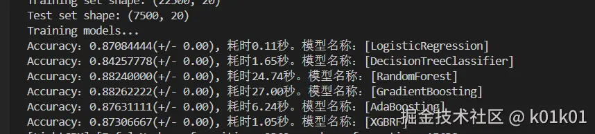
4. 多模型对比实验
模型配置详情
models = {
    'LogisticRegression': LogisticRegression(
        max_iter=2000,
        random_state=42,
        class_weight='balanced'
    ),
    'DecisionTreeClassifier': DecisionTreeClassifier(
        random_state=42,
        max_depth=10
    ),
    'RandomForest': RandomForestClassifier(
        n_estimators=100,
        random_state=42,
        class_weight='balanced'
    ),
    'GradientBoosting': GradientBoostingClassifier(
        n_estimators=100,
        random_state=42
    ),
    'AdaBoosting': AdaBoostClassifier(
        n_estimators=100,
        random_state=42
    ),
    'XGBRF': XGBRFClassifier(
        n_estimators=100,
        random_state=42
    ),
    'LGBM': LGBMClassifier(
        n_estimators=100,
        random_state=42,
        verbosity=-1
    )
}
模型评估方法
def evaluate_models(models, X, y, cv=5):
"""
全面评估模型性能
"""
results = {}
for name, clf in models.items():
start_time = time.time()
if name == 'LogisticRegression':
scores = cross_val_score(clf, train_x_scaled, train_y,
scoring='accuracy', cv=cv)
else:
scores = cross_val_score(clf, train_x, train_y,
scoring='accuracy', cv=cv)
end_time = time.time()
time_cost = end_time - start_time
results[name] = {
'mean_accuracy': scores.mean(),
'std_accuracy': scores.std(),
'time_cost': time_cost,
'scores': scores
}
print(f'模型: {name:20} | 准确率: {scores.mean():.6f} (±{scores.std():.4f}) | '
f'耗时: {time_cost:.2f}秒')
return results
5. 模型选择与超参数调优
选择LightGBM的原因
- 高准确率表现
- 训练速度快
- 内存消耗低
- 对类别特征友好
网格搜索调优
parameters = {
'colsample_bytree': [0.5, 0.7, 0.9],
'subsample': [0.6, 0.8, 1.0],
'reg_alpha': [0, 0.1, 0.5],
'reg_lambda': [0, 0.1, 0.5]
}
gsearch = GridSearchCV(
estimator=LGBMClassifier(
max_depth=11,
subsample=0.5,
min_split_gain=0.01,
random_state=42,
n_estimators=200
),
param_grid=parameters,
scoring='accuracy',
cv=5,
n_jobs=-1,
verbose=1
)
gsearch.fit(train_x, train_y)
6. 最终模型训练与预测
最优参数模型
best_params = gsearch.best_params_
print(f"最优参数: {best_params}")
print(f"最佳交叉验证分数: {gsearch.best_score_:.6f}")
clf_lgb = LGBMClassifier(
max_depth=11,
colsample_bytree=best_params['colsample_bytree'],
subsample=best_params['subsample'],
reg_alpha=best_params['reg_alpha'],
reg_lambda=best_params['reg_lambda'],
min_split_gain=0.01,
random_state=42,
n_estimators=200
)
clf_lgb.fit(train_x, train_y)
预测与结果分析
predict_y = clf_lgb.predict(test_x)
predict_df = pd.DataFrame(predict_y, index=test_x.index, columns=['subscribe'])
predict_df = predict_df.reset_index()
predict_df['subscribe'] = predict_df['subscribe'].replace([0, 1], ['no', 'yes'])
yes_count = (predict_y == 1).sum()
no_count = (predict_y == 0).sum()
total_count = len(predict_y)
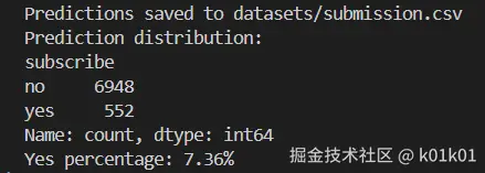
print("预测结果分布:")
print(f"认购客户(Yes): {yes_count} ({yes_count/total_count*100:.2f}%)")
print(f"未认购客户(No): {no_count} ({no_count/total_count*100:.2f}%)")
predict_df.to_csv('datasets/submission.csv', index=False)
print("预测结果已保存至: datasets/submission.csv")
运行结果
最终得分0.96


