

- input_tensor: 传入的张量
- axis: 维度, 默认计算所有维度
- keepdims: 如果为真保留维度, 默认为 False
- name: 数据名称
张量最大值
```reduce_max``函数可以帮助我们计算一个张量各个维度上元素的最大值.
格式:
tf.math.reduce_max(
    input_tensor, axis=None, keepdims=False, name=None
)
参数:
- input_tensor: 传入的张量
- axis: 维度, 默认计算所有维度
- keepdims: 如果为真保留维度, 默认为 False
- name: 数据名称
数据集分批
from_tensor_slices可以帮助我们切分传入 Tensor 的第一个维度. 得到的每个切片都是一个样本数据.
格式:
@staticmethod
from_tensor_slices(
    tensors
)
迭代
我们可以调用iter函数来生成迭代器.
格式:
iter(object[, sentinel])
参数:
-object: 支持迭代的集合对象
- sentinel: 如果传递了第二个参数, 则参数 object 必须是一个可调用的对象 (如, 函数). 此时, iter 创建了一个迭代器对象, 每次调用这个迭代器对象的
__next__()方法时, 都会调用 object
例子:
list = [1, 2, 3]
i = iter(list)
print(next(i))
print(next(i))
print(next(i))
输出结果:
1
2
3
截断正态分布
truncated_normal可以帮助我们生成一个截断的正态分布. 生成的正态分布值会在两倍的标准差的范围之内.
格式:
tf.random.truncated_normal(
    shape, mean=0.0, stddev=1.0, dtype=tf.dtypes.float32, seed=None, name=None
)
参数:
- shape: 张量的形状
- mean: 正态分布的均值, 默认 0.0
- stddev: 正态分布的标准差, 默认为 1.0
- dtype: 数据类型, 默认为 float32
- seed: 随机数种子
- name: 数据名称
relu 激活函数
激活函数有 sigmoid, maxout, relu 等等函数. 通过激活函数我们可以使得各个层之间达成非线性关系.
激活函数可以帮助我们提高模型健壮性, 提高非线性表达能力, 缓解梯度消失问题.
one_hot
tf.one_hot函数是讲 input 准换为 one_hot 类型数据输出. 相当于将多个数值联合放在一起作为多个相同类型的向量.
格式:
tf.one_hot(
    indices, depth, on_value=None, off_value=None, axis=None, dtype=None, name=None
)
参数:
- indices: 索引的张量
- depth: 指定独热编码维度的标量
- on_value: 索引 indices[j] = i 位置处填充的标量,默认为 1
- off_value: 索引 indices[j] != i 所有位置处填充的标量, 默认为 0
- axis: 填充的轴, 默认为 -1 (最里面的新轴)
- dtype: 输出张量的数据格式
- name:数据名称
assign_sub
assign_sub可以帮助我们实现张量自减.
格式:
tf.compat.v1.assign_sub(
    ref, value, use_locking=None, name=None
)
参数:
- ref: 多重张量
- value: 张量
- use_locking: 锁
- name: 数据名称
准备工作
import tensorflow as tf

# 定义超参数
batch_size = 256  # 一次训练的样本数目
learning_rate = 0.001  # 学习率
iteration_num = 20  # 迭代次数

# 读取mnist数据集
(x, y), _ = tf.keras.datasets.mnist.load_data()  # 读取训练集的特征值和目标值
print(x[:5])  # 调试输出前5个图
print(y[:5])  # 调试输出前5个目标值数字
print(x.shape)  # (60000, 28, 28) 单通道
print(y.shape)  # (60000,)

# 转换成常量tensor
x = tf.convert_to_tensor(x, dtype=tf.float32) / 255  # 转换为0~1的形式
y = tf.convert_to_tensor(y, dtype=tf.int32)  # 转换为整数形式

# 调试输出范围
print(tf.reduce_min(x), tf.reduce_max(x))  # 0~1
print(tf.reduce_min(y), tf.reduce_max(y))  # 0~9

# 分割数据集
train_db = tf.data.Dataset.from_tensor_slices((x, y)).batch(batch_size)  # 256为一个batch
train_iter = iter(train_db)  # 生成迭代对象

# 定义权重和bias [256, 784] => [256, 256] => [256, 128] => [128, 10]
w1 = tf.Variable(tf.random.truncated_normal([784, 256], stddev=0.1))  # 标准差为0.1的截断正态分布
b1 = tf.Variable(tf.zeros([256]))  # 初始化为0

w2 = tf.Variable(tf.random.truncated_normal([256, 128], stddev=0.1))  # 标准差为0.1的截断正态分布
b2 = tf.Variable(tf.zeros([128]))  # 初始化为0

w3 = tf.Variable(tf.random.truncated_normal([128, 10], stddev=0.1))  # 标准差为0.1的截断正态分布
b3 = tf.Variable(tf.zeros([10]))  # 初始化为0
输出结果:
[[[0 0 0 ... 0 0 0]
  [0 0 0 ... 0 0 0]
  [0 0 0 ... 0 0 0]
  ...
  [0 0 0 ... 0 0 0]
  [0 0 0 ... 0 0 0]
  [0 0 0 ... 0 0 0]]

 [[0 0 0 ... 0 0 0]
  [0 0 0 ... 0 0 0]
  [0 0 0 ... 0 0 0]
  ...
  [0 0 0 ... 0 0 0]
  [0 0 0 ... 0 0 0]
  [0 0 0 ... 0 0 0]]

 [[0 0 0 ... 0 0 0]
  [0 0 0 ... 0 0 0]
  [0 0 0 ... 0 0 0]
  ...
  [0 0 0 ... 0 0 0]
  [0 0 0 ... 0 0 0]
  [0 0 0 ... 0 0 0]]

 [[0 0 0 ... 0 0 0]
  [0 0 0 ... 0 0 0]
  [0 0 0 ... 0 0 0]
  ...
  [0 0 0 ... 0 0 0]
  [0 0 0 ... 0 0 0]
  [0 0 0 ... 0 0 0]]

 [[0 0 0 ... 0 0 0]
  [0 0 0 ... 0 0 0]
  [0 0 0 ... 0 0 0]
  ...
  [0 0 0 ... 0 0 0]
  [0 0 0 ... 0 0 0]
  [0 0 0 ... 0 0 0]]]
[5 0 4 1 9]
(60000, 28, 28)
(60000,)
tf.Tensor(0.0, shape=(), dtype=float32) tf.Tensor(1.0, shape=(), dtype=float32)
tf.Tensor(0, shape=(), dtype=int32) tf.Tensor(9, shape=(), dtype=int32)
train 函数
def train(epoch):  # 训练
    for step, (x, y) in enumerate(train_db):  # 每一批样本遍历
        # 把x平铺 [256, 28, 28] => [256, 784]
        x = tf.reshape(x, [-1, 784])

        with tf.GradientTape() as tape:  # 自动求解
            # 第一个隐层 [256, 784] => [256, 256]
            # [256, 784]@[784, 256] + [256] => [256, 256] + [256] => [256, 256] + [256, 256] (广播机制)
            h1 = x @ w1 + tf.broadcast_to(b1, [x.shape[0], 256])
            h1 = tf.nn.relu(h1)  # relu激活

            # 第二个隐层 [256, 256] => [256, 128]
            h2 = h1 @ w2 + b2
            h2 = tf.nn.relu(h2)  # relu激活

            # 输出层 [256, 128] => [128, 10]
            out = h2 @ w3 + b3

            # 计算损失MSE(Mean Square Error)
            y_onehot = tf.one_hot(y, depth=10)  # 转换成one_hot编码
            loss = tf.square(y_onehot - out)  # 计算总误差
            loss = tf.reduce_mean(loss)  # 计算平均误差MSE


        # 计算梯度
        grads = tape.gradient(loss, [w1, b1, w2, b2, w3, b3])

        # 更新权重
        w1.assign_sub(learning_rate * grads[0])  # 自减梯度*学习率
        b1.assign_sub(learning_rate * grads[1])  # 自减梯度*学习率
        w2.assign_sub(learning_rate * grads[2])  # 自减梯度*学习率
        b2.assign_sub(learning_rate * grads[3])  # 自减梯度*学习率
        w3.assign_sub(learning_rate * grads[4])  # 自减梯度*学习率
        b3.assign_sub(learning_rate * grads[5])  # 自减梯度*学习率

        if step % 100 == 0:  # 每运行100个批次, 输出一次
            print("epoch:", epoch, "step:", step, "loss:", float(loss))
run 函数
def run():
    for i in range(iteration_num):  # 迭代20次
        train(i)
完整代码
import tensorflow as tf
# 定义超参数
batch_size = 256 # 一次训练的样本数目
learning_rate = 0.001 # 学习率
iteration_num = 20 # 迭代次数
# 读取mnist数据集
(x, y), _ = tf.keras.datasets.mnist.load_data() # 读取训练集的特征值和目标值
print(x[:5]) # 调试输出前5个图
print(y[:5]) # 调试输出前5个目标值数字
print(x.shape) # (60000, 28, 28) 单通道
print(y.shape) # (60000,)
# 转换成常量tensor
x = tf.convert_to_tensor(x, dtype=tf.float32) / 255 # 转换为0~1的形式
y = tf.convert_to_tensor(y, dtype=tf.int32) # 转换为整数形式
# 调试输出范围
print(tf.reduce_min(x), tf.reduce_max(x)) # 0~1
print(tf.reduce_min(y), tf.reduce_max(y)) # 0~9
# 分割数据集
train_db = tf.data.Dataset.from_tensor_slices((x, y)).batch(batch_size) # 256为一个batch
train_iter = iter(train_db) # 生成迭代对象
# 定义权重和bias [256, 784] => [256, 256] => [256, 128] => [128, 10]
w1 = tf.Variable(tf.random.truncated_normal([784, 256], stddev=0.1)) # 标准差为0.1的截断正态分布
b1 = tf.Variable(tf.zeros([256])) # 初始化为0
w2 = tf.Variable(tf.random.truncated_normal([256, 128], stddev=0.1)) # 标准差为0.1的截断正态分布
b2 = tf.Variable(tf.zeros([128])) # 初始化为0
w3 = tf.Variable(tf.random.truncated_normal([128, 10], stddev=0.1)) # 标准差为0.1的截断正态分布
b3 = tf.Variable(tf.zeros([10])) # 初始化为0
def train(epoch): # 训练
for step, (x, y) in enumerate(train_db): # 每一批样本遍历
# 把x平铺 [256, 28, 28] => [256, 784]
x = tf.reshape(x, [-1, 784])
with tf.GradientTape() as tape: # 自动求解
# 第一个隐层 [256, 784] => [256, 256]
# [256, 784]@[784, 256] + [256] => [256, 256] + [256] => [256, 256] + [256, 256] (广播机制)
h1 = x @ w1 + tf.broadcast_to(b1, [x.shape[0], 256])
h1 = tf.nn.relu(h1) # relu激活
# 第二个隐层 [256, 256] => [256, 128]
h2 = h1 @ w2 + b2
h2 = tf.nn.relu(h2) # relu激活

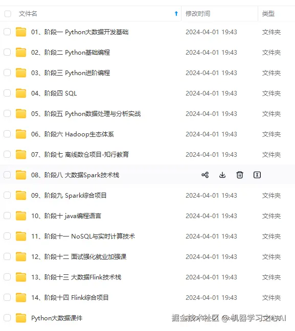
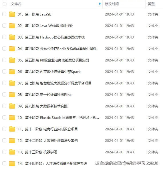
**既有适合小白学习的零基础资料,也有适合3年以上经验的小伙伴深入学习提升的进阶课程,涵盖了95%以上大数据知识点,真正体系化!**
**由于文件比较多,这里只是将部分目录截图出来,全套包含大厂面经、学习笔记、源码讲义、实战项目、大纲路线、讲解视频,并且后续会持续更新**
**[需要这份系统化资料的朋友,可以戳这里获取](https://gitee.com/vip204888)**
