Transformation变换

63 阅读1分钟

Model Transform 模型变换

2D变换

Linear Transformation 线性变换

x=ax+byx'=ax+by

y=cx+dyy'=cx+dy

矩阵形式为

[xy]=[abcd][xy]\begin{bmatrix}x'\\y\end{bmatrix}=\begin{bmatrix}a&b\\c&d\end{bmatrix}\begin{bmatrix}x\\y\end{bmatrix}

Scale Matrix 缩放

[sxxsyy]=[sx00sy][xy]\begin{bmatrix}s_xx\\s_yy\end{bmatrix}=\begin{bmatrix}s_x&0\\0&s_y\end{bmatrix}\begin{bmatrix}x\\y\end{bmatrix}

Reflection Matrix 镜像

Horizontal reflection:

[xy]=[1001][xy]\begin{bmatrix}-x\\y\end{bmatrix}=\begin{bmatrix}-1&0\\0&1\end{bmatrix}\begin{bmatrix}x\\y\end{bmatrix}

Shear Matrix 切变

Horizontal shift:

[x+ay]=[1a01][xy]\begin{bmatrix}x+a\\y\end{bmatrix}=\begin{bmatrix}1&a\\0&1\end{bmatrix}\begin{bmatrix}x\\y\end{bmatrix}

Rotate 旋转

默认绕原点(0,0)(0,0)逆时针方向(counterclockwise)旋转

Rθ=[cosθsinθsinθcosθ]R_{\theta}=\begin{bmatrix}cos\theta&-sin\theta\\sin\theta&cos\theta\end{bmatrix}

推导:

rotate.png

Translation 平移

x=x+txx'=x+t_x

y=y+tyy'=y+t_y

这个变换无法直接写为统一的矩阵形式

[xy]=[abcd][xy]+[txty]\begin{bmatrix}x'\\y\end{bmatrix}=\begin{bmatrix}a&b\\c&d\end{bmatrix}\begin{bmatrix}x\\y\end{bmatrix}+\begin{bmatrix}t_x\\t_y\end{bmatrix}

因为平移不是线性变换

但是为了变换的形式的统一,可以引入齐次坐标(homogeneous coordinates)来表示

齐次坐标

对于二维向量,增加一个维度ww

2D Point = (x,y,1)T(x,y,1)^T

2D Vector =(x,y,0)T(x,y,0)^T

在矩阵运算时

[xyw]=[10tx01ty001][xy1]=[x+txy+ty1]\begin{bmatrix}x'\\y'\\w'\end{bmatrix} = \begin{bmatrix}1&0&t_x\\0&1&t_y\\0&0&1\end{bmatrix} \cdot \begin{bmatrix}x\\y\\1\end{bmatrix} = \begin{bmatrix}x+t_x\\y+t_y\\1\end{bmatrix}

同时,增加的维度在运算时也具有意义

对于[xyw]\begin{bmatrix}x\\y\\w\end{bmatrix},在ww不为0时,表示为一个点,标准化运算后为[x/wy/w1]\begin{bmatrix}x/w\\y/w\\1\end{bmatrix}

  • vector + vector = vector
  • point - point = vector
  • point + vector = point
  • point + point = ??

对于最后一种情况,得到的也是一个点,在进行标准化运算后,得到的是两点的中点

引入齐次坐标的目的是能够使用一个矩阵乘一个向量来表示所有变换

以上[xy]=[abcd][xy]+[txty]\begin{bmatrix}x'\\y\end{bmatrix}=\begin{bmatrix}a&b\\c&d\end{bmatrix}\begin{bmatrix}x\\y\end{bmatrix}+\begin{bmatrix}t_x\\t_y\end{bmatrix}形式的变换,统称为仿射变换(Affine Transformations)

用齐次坐标的形式来表示

[xy1]=[abtxcdty001][xy1]\begin{bmatrix}x'\\y'\\1\end{bmatrix} = \begin{bmatrix}a&b&t_x\\c&d&t_y\\0&0&1\end{bmatrix} \cdot \begin{bmatrix}x\\y\\1\end{bmatrix}

Scale

S(sx,sy)=[sx000sy0001]S(s_x,s_y)=\begin{bmatrix}s_x&0&0\\0&s_y&0\\0&0&1\end{bmatrix}

Rotation

R(θ)=[cosθsinθ0sinθcosθ0001]R(\theta)=\begin{bmatrix}cos\theta&-sin\theta&0\\sin\theta&cos\theta&0\\0&0&1\end{bmatrix}

Translation

T(tx,ty)=[10tx01ty001]T(t_x,t_y)=\begin{bmatrix}1&0&t_x\\0&1&t_y\\0&0&1\end{bmatrix}

Inverse Transform 逆变换

逆矩阵M1M^{-1},即做与矩阵MM相反的变换

Composing Transform 组合变换

因为矩阵运算具有结合律,不同类型的变换可以通过多个矩阵相乘合成为一个变换矩阵。但需要注意矩阵运算不满足交换律,因此变换是具有顺序的,例如先旋转再平移、先平移再旋转可能会得到不同的结果。

在使用多个矩阵进行变换时,变换是从右向左应用的

例如T(1,0)R45°[xy1]T_{(1,0)}\cdot R_{45\degree}\cdot\begin{bmatrix}x\\y\\1\end{bmatrix}中,先进行Rotate变换,再进行Translate变换

通过预先将多个矩阵变换合成为一个矩阵,可以在运算时提高性能

Decomposing Complex Transforms 分解变换

如何绕任意一个点进行旋转变换?

由于我们定义的旋转矩阵是绕原点进行旋转的,可以先将这个点移动到原点,进行旋转变换后,再进行一次平移还原到原来的位置。可表示为T(c)R(α)T(c)T(c)\cdot R(\alpha)\cdot T(-c)

旋转变换的一些性质

对于旋转矩阵Rθ=[cosθsinθsinθcosθ]R_{\theta}=\begin{bmatrix}cos\theta&-sin\theta\\sin\theta&cos\theta\end{bmatrix}

若旋转角度为θ-\theta,则有Rθ=[cosθsinθsinθcosθ]=RθTR_{-\theta}=\begin{bmatrix}cos\theta&sin\theta\\-sin\theta&cos\theta\end{bmatrix}=R_{\theta}^{T}

即旋转θ-\theta是旋转θ\theta的转置,而通过定义我们可以知道旋转θ-\theta与旋转θ\theta是互逆的操作,有Rθ=Rθ1R_{-\theta}=R_{\theta}^{-1}

由此可得RθT=Rθ1R_{\theta}^T=R_{\theta}^{-1},旋转矩阵的逆矩阵等于转置矩阵

在数学中,如果一个矩阵的逆等于转置,称这个矩阵为正交矩阵

3D变换

3D Point = (x,y,z,1)T(x,y,z,1)^T

3D Vector =(x,y,z,0)T(x,y,z,0)^T

(x,y,z,w)(x,y,z,w)三维向量,ww不为0时即为三维空间中一点(x/w,y/w,z/w)(x/w,y/w,z/w)

3D 仿射变换

[xyz1]=[abctxdeftyghitz0001][xyz1]\begin{bmatrix}x'\\y'\\z'\\1\end{bmatrix} = \begin{bmatrix}a&b&c&t_x\\d&e&f&t_y\\g&h&i&t_z\\0&0&0&1\end{bmatrix} \cdot \begin{bmatrix}x\\y\\z\\1\end{bmatrix}

应用这个矩阵时,先进行线性变换,再进行平移

Scale

S(sx,sy,sz)=[sx0000sy0000sz00001]S(s_x,s_y,s_z)=\begin{bmatrix}s_x&0&0&0\\0&s_y&0&0\\0&0&s_z&0\\0&0&0&1\end{bmatrix}

Translation

T(tx,ty,tz)=[100tx010ty001tz0001]T(t_x,t_y,t_z)=\begin{bmatrix}1&0&0&t_x\\0&1&0&t_y\\0&0&1&t_z\\0&0&0&1\end{bmatrix}

Rotation(x-, y-,z- axis)

Rx(θ)=[10000cosθsinθ00sinθcosθ00001]R_x(\theta)=\begin{bmatrix}1&0&0&0\\0&cos\theta&-sin\theta&0\\0&sin\theta&cos\theta&0\\0&0&0&1\end{bmatrix}

Ry(θ)=[cosθ0sinθ00100sinθ0cosθ00001]R_y(\theta)=\begin{bmatrix}\cos\theta&0&sin\theta&0\\0&1&0&0\\-sin\theta&0&cos\theta&0\\0&0&0&1\end{bmatrix}

Rz(θ)=[cosθsinθ00sinθcosθ0000100001]R_z(\theta)=\begin{bmatrix}cos\theta&-sin\theta&0&0\\sin\theta&cos\theta&0&0\\0&0&1&0\\0&0&0&1\end{bmatrix}

Euler angles 欧拉角

对三维空间中的旋转,可以用分别绕x,y,z轴的三个旋转组合而成

Rxyz(α,β,γ)=Rx(α)Ry(β)Rz(γ)R_{xyz}(\alpha,\beta,\gamma)=R_x{(\alpha)}R_y{(\beta)}R_z{(\gamma)}

通常把三个分量称为roll,pitch,yaw

但是欧拉角旋转在两个轴重合时,会出现失去一个自由度的情况,称为万向节死锁

Rodrigues' Rotation Formula

绕任意轴axisaxis旋转α\alpha角度的公式,轴axisaxis是默认经过原点的

(n,α)=cos(α)I=(1cos(α))nnT+sin(α)N(\bold{n},\alpha)=cos(\alpha)I=(1-cos(\alpha))\bold{n}\bold{n}^T+sin(\alpha)\bold{N}

N=[0nznynz0nxnynx0]\bold{N}=\begin{bmatrix}0&-n_z&n_y\\n_z&0&-n_x\\-n_y&n_x&0\end{bmatrix}

Quaternion 四元数旋转

能够应用于插值运算

留个坑详解四元数(未完成)

View Transform 观测变换

进行观测变换需要大量信息,包括:摄像机的位置和朝向、投影的类型、视场的大小( FOV field of view)、渲染的分辨率

通常可以把观测变换分解为三个流程

  • Camera Transform 相机变换
  • Projection Transform 投影变换
  • Viewport Transform 视口变换

在变换流程中坐标系统有特定的名称:

space.png

Figure 8.2 from Fundamentals of Computer Graphics, 5th Edition

一些别名

camera space也叫eye space,camera transformation也称作viewing transformation,canonical view volume也叫clip space或normalized device coordinates(NDC),screen space也叫pxiel coordinates

Fundamentals of Computer Graphics, 5th Edition P159

Camera Transform

相机变换将点转变为归一化坐标(canonical cooridnates)

定义一个相机变换:

  • Position e\vec{e}
  • Look-at/gaze direction g^\hat{g}
  • Up direction t^\hat{t}

由于运动是相对的,为了简化相机变换,我们可以把摄像机相对物体的运动看做物体相对摄像机的运动。把摄像机固定在原点,up朝向yy轴,look at朝向z-z

用变换来描述:

  1. 将摄像机移动到原点
  2. g^\hat{g}转到Z-Z
  3. t^\hat{t}转到YY
  4. (g^×t^)(\hat{g} \times \hat{t})转到XX

写成矩阵形式Mcam=RviewTviewM_{cam}=R_{view}T_{view}

Tview=[100xe010ye001ze0001]T_{view}=\begin{bmatrix}1&0&0&-x_e\\0&1&0&-y_e\\0&0&1&-z_e\\0&0&0&1\end{bmatrix}

将摄像机的坐标轴旋转到XYZXYZ轴方向并不容易求,但是我们可以将XYZXYZ旋转到摄像机的坐标轴方向得到逆矩阵,在上文我们证明了旋转矩阵的逆等于转置,由此可以求出RviewR_{view}

Rview1=[xg^×t^xtxg0yg^×t^ytyg0zg^×t^ztzg00001]R_{view}^{-1}=\begin{bmatrix}x_{\hat{g}\times\hat{t}}&x_t&x_{-g}&0\\y_{\hat{g}\times\hat{t}}&y_t&y_{-g}&0\\z_{\hat{g}\times\hat{t}}&z_t&z_{-g}&0\\0&0&0&1\end{bmatrix} Rview=[xg^×t^yg^×t^zg^×t^0xtytzt0xgygzg00001]R_{view}=\begin{bmatrix}x_{\hat{g}\times\hat{t}}&y_{\hat{g}\times\hat{t}}&z_{\hat{g}\times\hat{t}}&0\\x_t&y_t&z_t&0\\x_{-g}&y_{-g}&z_{-g}&0\\0&0&0&1\end{bmatrix}

合并后得到

Mcam=[xg^×t^yg^×t^zg^×t^xextytztyexgygzgze0001]M_{cam}=\begin{bmatrix}x_{\hat{g}\times\hat{t}}&y_{\hat{g}\times\hat{t}}&z_{\hat{g}\times\hat{t}}&-x_e\\x_t&y_t&z_t&-y_e\\x_{-g}&y_{-g}&z_{-g}&-z_e\\0&0&0&1\end{bmatrix}

Viewport Trasnform 视口变换

将经过camera transform变换后得到的NDC坐标绘制到大小为nx×nyn_x \times n_y像素大小的屏幕上,需要将NDC的标准正方形[1,1]2[-1,-1]^2映射到[0.5,nx0.5]×[0.5,ny0.5][-0.5, n_x-0.5] \times [-0.5, n_y-0.5]的矩形

4×34\times3的像素映射为[0.5,3.5]×[0.5,2.5][-0.5,3.5]\times[-0.5, 2.5]

raster.png

Figure 3.10 from Fundamentals of Computer Graphics, 5th Edition

写作矩阵形式: Mvp=[nx200nx120ny20ny1200100001]M_{vp}=\begin{bmatrix}\frac{n_x}{2}&0&0&\frac{n_x-1}{2}\\0&\frac{n_y}{2}&0&\frac{n_y-1}{2}\\0&0&1&0\\0&0&0&1\end{bmatrix}

此处暂时忽略了zz坐标,因为zz轴方向的距离并不会影响投影的位置。但在后续处理中会用到zz坐标来处理遮挡关系

Projection Transform 投影变换

Orthographic projection 正交投影

在空间中定义一个范围[l,r]×[b,t]×[f,n][l,r]\times[b,t]\times[f,n],称作orthographic view volume,将这个范围映射到一个[1,1]3[-1,1]^3的标准(canonical)立方体内

Mortho=[2rl00002tb00002nf00001][100r+l2010t+b2001n+f20001]=[2rl00l+rlr02tb0b+tbt002nff+nfn0001]M_{ortho}= \begin{bmatrix} \frac{2}{r-l}&0&0&0\\ 0&\frac{2}{t-b}&0&0\\ 0&0&\frac{2}{n-f}&0\\ 0&0&0&1 \end{bmatrix} \begin{bmatrix} 1&0&0&-\frac{r+l}{2}\\ 0&1&0&-\frac{t+b}{2}\\ 0&0&1&-\frac{n+f}{2}\\ 0&0&0&1\\ \end{bmatrix} = \begin{bmatrix} \frac{2}{r-l}&0&0&\frac{l+r}{l-r}\\ 0&\frac{2}{t-b}&0&\frac{b+t}{b-t}\\ 0&0&\frac{2}{n-f}&\frac{f+n}{f-n}\\ 0&0&0&1\\ \end{bmatrix}

在经过MvpM_{vp}MorthoM_{ortho}的组合变换后,一个点应该变为[xpixelypixelzcanonical1]\begin{bmatrix}x_{pixel}\\y_{pixel}\\z_{canonical}\\1\end{bmatrix}zz坐标仍然在[1,1][-1,1]范围内,之后会在深度缓冲中使用

Perspective Transform 透视变换

透视投影在空间中的范围称作Frustum

projection.png

Figure 8.13 from Fundamentals of Computer Graphics, 5th Edition

通过侧视图,我们可以推导出在进行透视投影后,yy轴方向的长度会变为ys=dzyy_s=\frac{d}{z}y

geometry.png

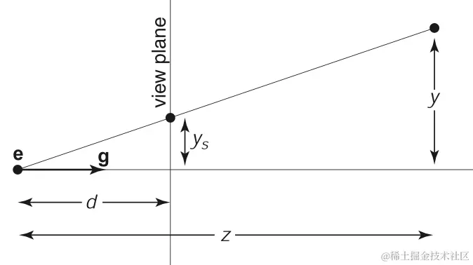
Figure 8.8 from Fundamentals of Computer Graphics, 5th Edition

zz坐标出现在了分母,导致我们不能直接使用纺射变换来推导透视投影矩阵

但是我们可以对齐次坐标运算进行推广,来实现在仿射变换中使用除法

先前我们规定用[xyz1]T\begin{bmatrix}x&y&z&1\end{bmatrix}^T来表示三维空间中的一点(x,y,z)(x,y,z),并且保证仿射变换矩阵的第四行始终为[0001]\begin{bmatrix}0&0&0&1\end{bmatrix}

现在我们可以定义将ww定义为x,y,zx,y,z坐标的分母,用齐次坐标[xyzw]T\begin{bmatrix}x&y&z&w\end{bmatrix}^T来表示带点(x/w,y/w,z/w)(x/w,y/w,z/w),也就是将(x,y,z,w)(x,y,z,w)各分量同时除以ww,0项仍然为0,得到(x/w,y/w,z/w1)(x/w,y/w,z/w,1)。这个操作称为齐次除法透视除法。这样我们就可以在矩阵的第四行使用任意值来支持更广泛的变换

具体来说,线性变换允许我们实现

x=ax+by+czx'=ax+by+cz

仿射变换将变换扩展为

x=ax+by+c+dx'=ax+by+c+d

ww定义为分母就可以实现计算

x=ax+by+cz+dex+fy+gz+hx'=\frac{ax+by+cz+d}{ex+fy+gz+h}

这种变换可以称作线性有理函数,但是一个额外的约束条件是,坐标每个分量的分母都是相同的

x=a1x+b1y+c1z+d1ex+fy+gz+hx'=\frac{a_1x+b_1y+c_1z+d_1}{ex+fy+gz+h}

y=a2x+b2y+c2z+d2ex+fy+gz+hy'=\frac{a_2x+b_2y+c_2z+d_2}{ex+fy+gz+h}

z=a3x+b3y+c3z+d3ex+fy+gz+hz'=\frac{a_3x+b_3y+c_3z+d_3}{ex+fy+gz+h}

将这些变换合并为一个矩阵

[x~y~z~w~]=[a1b1c1d1a2b2c2d2a3b3c3d3efgh]=[xyz1]\begin{bmatrix} \tilde{x}\\\tilde{y}\\\tilde{z}\\\tilde{w} \end{bmatrix} = \begin{bmatrix} a_1&b_1&c_1&d_1\\ a_2&b_2&c_2&d_2\\ a_3&b_3&c_3&d_3\\ e&f&g&h \end{bmatrix} = \begin{bmatrix} x\\y\\z\\1 \end{bmatrix}

对于这个变换矩阵MM,与任意的常数kk相乘不会改变结果

Perspective Projection 透视投影

在透视投影中,我们将采用惯例,将摄像机放在原点,朝向z-z方向,所以任意一点(x,y,z)(x,y,z)到摄像机的距离为z-z;将近裁剪平面作为投影平面,所以投影平面的距离为n-n(n < 0)

透视投影也可以分解为两个步骤,先将投影区域Frustum压缩成正交投影中的轴对齐的一个四方柱体,再进行正交投影

通过侧视图和俯视图,利用三角形相似进行推导,可以得到[xyz1][nx/zny/zunknown1]==[nxnyunknownn]\begin{bmatrix}x\\y\\z\\1\end{bmatrix}\Rightarrow\begin{bmatrix}nx/z\\ny/z\\unknown\\1\end{bmatrix}==\begin{bmatrix}nx\\ny\\unknown\\n\end{bmatrix}

将齐次除法还原,[nxnyunknownz]\begin{bmatrix}nx\\ny\\unknown\\z\end{bmatrix},此时已经够推导出矩阵的一部分

Mpersportho=[n0000n00????0010]M_{persp\rightarrow ortho}=\begin{bmatrix}n&0&0&0\\0&n&0&0\\?&?&?&?\\0&0&1&0\end{bmatrix}

再考虑一些特殊点:

  • 近平面上的点在压缩后不会发生变化,[xyn1][xyn1]==[nxnyn2n]\begin{bmatrix}x\\y\\n\\1\end{bmatrix}\Rightarrow\begin{bmatrix}x\\y\\n\\1\end{bmatrix}==\begin{bmatrix}nx\\ny\\n^2\\n\end{bmatrix},考虑MpersporthoM_{persp\rightarrow ortho}矩阵中的第三行与这个坐标相乘,得到了n2n^2,显然与x,yx,y无关,由此可以得出第三行的前两项为0,利用待定系数法设第三行为[00AB]\begin{bmatrix}0&0&A&B\end{bmatrix},有An+B=n2An+B=n^2

  • 远平面上的点在压缩后zz坐标不会改变,我们已经得出第三行与x,yx,y无关,所以取远平面的中心点来计算[00f1][00f1]==[00f2f]\begin{bmatrix}0\\0\\f\\1\end{bmatrix}\Rightarrow\begin{bmatrix}0\\0\\f\\1\end{bmatrix}==\begin{bmatrix}0\\0\\f^2\\f\end{bmatrix},根据设出的值可以得到Af+B=f2Af+B=f^2

于是有方程组{An+B=n2Af+B=f2\begin{cases}An+B=n^2\\Af+B=f^2\end{cases} 解得:{A=n+fB=nf\begin{cases}A=n+f\\B=-nf\end{cases}

最终我们得到

Mpersportho=[n0000n0000n+fnf0010]M_{persp\rightarrow ortho}=\begin{bmatrix}n&0&0&0\\0&n&0&0\\0&0&n+f&-nf\\0&0&1&0\end{bmatrix}
Mpersp=Mpersportho=[2nrl0l+rlr002ntbb+tbt000n+fnf2fnfn0010]M_{persp}=M_{persp\rightarrow ortho}= \begin{bmatrix} \frac{2n}{r-l}&0&\frac{l+r}{l-r}&0\\ 0&\frac{2n}{t-b}&\frac{b+t}{b-t}&0\\ 0&0&\frac{n+f}{n-f}&\frac{2fn}{f-n}\\ 0&0&1&0\\ \end{bmatrix}

OpenGL使用的矩阵

MOpenGL=[2nrl0l+rlr002ntbb+tbt000n+fnf2fnfn0010]M_{OpenGL}= \begin{bmatrix} \frac{2|n|}{r-l}&0&\frac{l+r}{l-r}&0\\ 0&\frac{2|n|}{t-b}&\frac{b+t}{b-t}&0\\ 0&0&\frac{|n|+|f|}{|n|-|f|}&\frac{2|f||n|}{|f|-|n|}\\ 0&0&-1&0\\ \end{bmatrix}

投影变换的流程

compute MvpM_{vp}

compute MperspM_{persp}

compute McamM_{cam}

M=MvpMperspMcamM=M_{vp}M_{persp}M_{cam}

MM传入顶点着色器计算

参考资料

Fundamentals of Computer Graphics, 5th Edition

GAMES101 Lecture03-04