一、酒驾风险行为分析预测

1.背景描述

本数据集来自2007年青少年风险行为监测系统（YRBSS），该系统是由美国疾病控制和预防中心（CDC）进行的年度调查，旨在监测有健康风险的青少年行为的流行情况。
本数据集的重点是青少年最近（在过去30天内）是否乘坐过醉酒司机的车。

2.数据说明

本数据集包含13387条记录，涉及以下6个变量：

• 是否在过去30天内与饮酒驾驶者一起乘车：1=有；0=没有
• 是否是女性：1=女性；0=男性
• 就读年级：9，10，11，12
• 年龄
• 是否吸烟：1=是；0=否
• 是否拥有驾照：1=有；0=没有

3.数据来源

www.kaggle.com/datasets/ut…

二、数据分析

1.数据读取

import pandas as pd
df=pd.read_csv('data/data225503/Risky_behavior_in_youths.csv',encoding='gbk')
df.head()

2.空值处理

df.isnull().sum()

序号                       0
是否在过去30天内与饮酒驾驶者一起乘车      0
是否是女性                  755
就读年级                    67
年龄                      54
是否吸烟                   388
是否拥有驾照                  54
dtype: int64

df.shape

(13387, 7)

df.isnull().sum()/df.shape[0]

序号                     0.000000
是否在过去30天内与饮酒驾驶者一起乘车    0.000000
是否是女性                  0.056398
就读年级                   0.005005
年龄                     0.004034
是否吸烟                   0.028983
是否拥有驾照                 0.004034
dtype: float64

df.dropna(inplace=True)
df.drop(['序号'], inplace=True, axis=1)
df.shape

(12282, 6)

df.describe()

从上表可以看出，

• 经过清洗后，共有12282条数据；
• 在过去30天内与饮酒驾驶者一起乘车占比31.34%；
• 数据中女生人数多于男生，女生人数占比52%；
• 数据中大部分的年级为10、11；
• 年龄均值为16岁；
• 数据中吸烟和有驾照的人为多数，占比分别为53%和67%。

三、数据预处理

1.数据归一化

columns = df.columns
print(columns)

Index(['是否在过去30天内与饮酒驾驶者一起乘车', '是否是女性', '就读年级', '年龄', '是否吸烟', '是否拥有驾照'], dtype='object')

for column in columns[1:]:
    col = df[column]
    col_min = col.min()
    col_max = col.max()
    normalized = (col - col_min) / (col_max - col_min)
    df[column] = normalized

df.head()

2.数据集切分

from sklearn.model_selection import train_test_split

# 切分数据集为 训练集 、 测试集
train, test = train_test_split(df, test_size=0.2, random_state=2023)

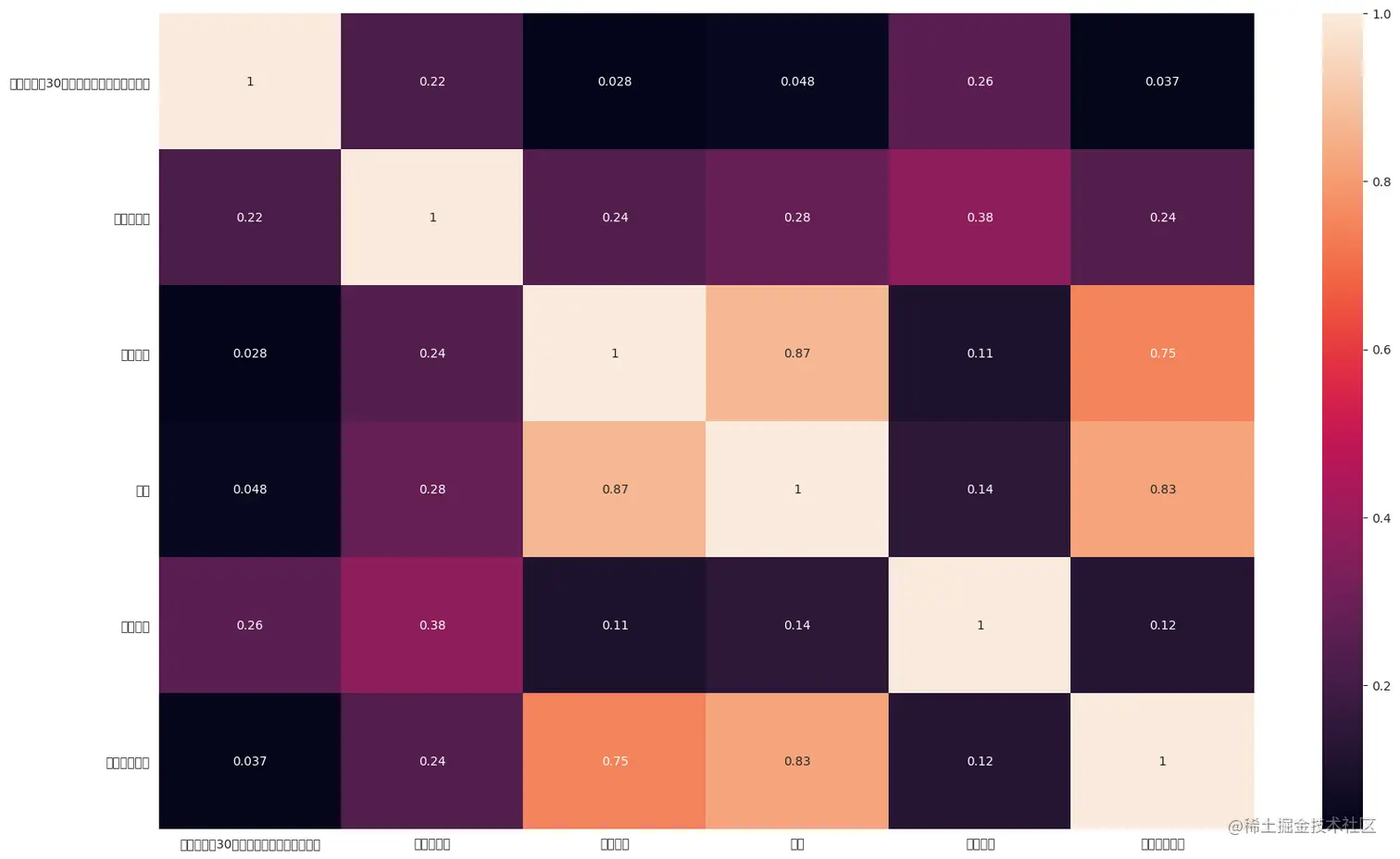
3.协相关

df.corr()

import matplotlib.pyplot as plt
%matplotlib inline
import seaborn as sns
sns.set_style('whitegrid')

# 热力图
plt.figure(figsize=(20,12))
sns.heatmap(df.corr(), annot=True)

四、模型训练

1.网络定义

import paddle
import paddle.nn.functional as F

# 定义动态图
class Net(paddle.nn.Layer):
    def __init__(self):
        super(Net, self).__init__()
        # 定义一层全连接层，输出维度是1，激活函数为None，即不使用激活函数
        self.fc = paddle.nn.Linear(in_features=5,out_features=2)
    
    # 网络的前向计算函数
    def forward(self, inputs):
        pred = self.fc(inputs)
        return pred

2.超参设置

net=Net()
# 设置迭代次数
epochs = 6
#  paddle.nn.loss.CrossEntropyLoss正常
#  paddle.nn.CrossEntropyLoss不正常
loss_func = paddle.nn.CrossEntropyLoss()
#优化器
opt = paddle.optimizer.Adam(learning_rate=0.1,parameters=net.parameters())

3.模型训练

#训练程序
for epoch in range(epochs):
    all_acc = 0
    for i in range(train.shape[0]):
        x = paddle.to_tensor([train.iloc[i,1:]])
        y = paddle.to_tensor([train.iloc[i,0]])
        infer_y = net(x)
        loss = loss_func(infer_y,y)
        loss.backward()
        y=label = paddle.to_tensor([y], dtype="int64")
        acc= paddle.metric.accuracy(infer_y, y)
        all_acc=all_acc+acc.numpy()
        opt.step()
        opt.clear_gradients#清除梯度
        # print("epoch: {}, loss is: {},acc is:{}".format(epoch, loss.numpy(),acc.numpy()))  #由于输出过长，这里注释掉了
    print("第{}次正确率为：{}".format(epoch+1,all_acc/i))

第1次正确率为：[0.6094259]
第2次正确率为：[0.6070847]
第3次正确率为：[0.5988396]
第4次正确率为：[0.61268324]
第5次正确率为：[0.61115634]
第6次正确率为：[0.5905945]

五、模型评估

1.模型训练

#测试集数据运行
net.eval()#模型转换为测试模式
all_acc = 0
for i in range(test.shape[0]):
        x = paddle.to_tensor([test.iloc[i,:-1]])
        y = paddle.to_tensor([test.iloc[i,-1]])        
        infer_y = net(x)
        y=label = paddle.to_tensor([y], dtype="int64")
    # 计算损失与精度
        loss = loss_func(infer_y, y)
        acc = paddle.metric.accuracy(infer_y, y)
        all_acc = all_acc+acc.numpy()
    # 打印信息
        #print("loss is: {}, acc is: {}".format(loss.numpy(), acc.numpy()))
print("测试集正确率：{}".format(all_acc/i))

测试集正确率：[0.44177523]

2.预测

import numpy as np

#预测结果展示
net.eval()
x = paddle.to_tensor([test.iloc[0,1:]])
y = paddle.to_tensor([test.iloc[0,0]])    
infer_y = net(x)
y=label = paddle.to_tensor([y], dtype="int64")
# 计算损失与精度
loss = loss_func(infer_y, y)
# 打印信息
print("test[0] is :\n{}\n y_test[0] is :{}\n predict is {}".format(test.iloc[0,1:] ,test.iloc[0,0], np.argmax(infer_y.numpy()[0])))

test[0] is :
是否是女性     0.00
就读年级      1.00
年龄        0.75
是否吸烟      1.00
是否拥有驾照    1.00
Name: 481, dtype: float64
 y_test[0] is :0
 predict is 0