Application

• stock market forecast
• self-driving car
• recommendation

Step 1: Model

Linear model: $y = b + \sum_i w_i x_i$

Step 2: Goodness of Function

Loss function $L$

Input: a function

Output: how bad it is

Regularization

• smooth functions are preferred (smaller $w_i$ -> smaller change when $x$ changes) - not sensitive to noise
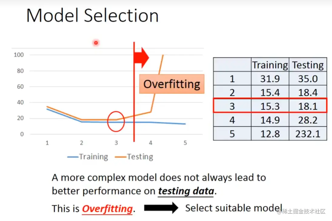
• larger $\lambda$ -> larger training error, not necessarily smaller testing error
• How smooth? -> select $\lambda$ obtaining the best model
• bias should not be considered in regularization （只提供位移，与smooth无关）

Step3: Gradiend Descent

Consider $L(w)$

• (Randomly) pick an initial value $w^0$
• Compute $\frac{dL}{dw}|_{w=w^0}$, $w^1 = w^0 - \eta \frac{dL}{dw}|_{w=w^0}$
• Repeat -> local optimal

Two parameters $L(w, b)$

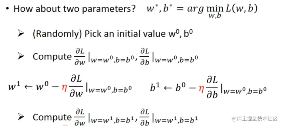
Gradient: $\nabla L = \begin{bmatrix} \frac{\partial L}{\partial w} \\ \\ \frac{\partial L}{\partial b} \end{bmatrix}$