

开启掘金成长之旅!这是我参与「掘金日新计划 · 2 月更文挑战」的第 32 天,点击查看活动详情
(本文是第34篇活动文章)
6. EM
简而言之:是一种优化算法。 一般用于MLE(最大似然估计)问题,估计参数。 根据已知的观察结果 ,通过 maximum likelihood principle 导出我们觉得最合理的 model(也称为 identification)。
一种trick就是增加隐变量: 这种问题常用stochastic sampling (Monte Carlo methods)、用一些假设来绕过计算,或用variational inference
6.1 EM算法介绍
EM算法解决含有隐变量 (hidden variable) 的概率模型参数的极大似然估计,每次迭代由两步组成: E步, 求期望 (expectation) M步, 使期望最大化 (maximization) 所以这一算法称为期望极大算法 (expectation maximization algorithm) ,简称EM算法。
6.1.1 最小化KL散度视角
EM算法的原理是最小化KL散度。
有监督场景下的最大似然估计:
如果只给出X,那么Y就是隐变量
举例:GMM模型
不用是因为两项都难估计。
易得(分类问题)
:这些X都属于同一类,所以应该长得差不多→假设为正态分布
只知道 是隐变量
(是统计频率)(没看懂和的区别)
\begin{aligned}
&KL\big(\tilde{p}(X,Y)||p_\theta(X,Y)\big)\\
&=\sum_{X,Y}\tilde{p}(X,Y)\log\frac{\tilde{p}(X,Y)}{p_\theta(X,Y)}\\
&=\sum_{X,Y}\tilde{p}(X)\tilde{p}(Y|X)\log\frac{\tilde{p}(Y|X)\tilde{p}(X)}{p_\theta(X|Y)p_\theta(Y)}\\
&=\sum_{X}\tilde{p}(X)\sum_Y\tilde{p}(Y|X)\log\frac{\tilde{p}(Y|X)\tilde{p}(X)}{p_\theta(X|Y)p_\theta(Y)}\\
&=\mathbb{E}_X\Bigg[\sum_Y\tilde{p}(Y|X)\log\frac{\tilde{p}(Y|X)\tilde{p}(X)}{p_\theta(X|Y)p_\theta(Y)}\Bigg]\\
&=\mathbb{E}_X\Bigg[\sum_Y\tilde{p}(Y|X)\log\frac{\tilde{p}(Y|X)}{p_\theta(X|Y)p_\theta(Y)}+\sum_Y\tilde{p}(Y|X)\log\tilde{p}(X)\Bigg](对数乘法)\\
&=\mathbb{E}_X\Bigg[\sum_Y\tilde{p}(Y|X)\log\frac{\tilde{p}(Y|X)}{p_\theta(X|Y)p_\theta(Y)}\Bigg]+\mathbb{E}\big[\log\tilde{p}(X)\big]
\end{aligned}$$
$\mathbb{E}\big[\log\tilde{p}(X)\big]$是常数,所以只需要优化第一项式,使$KL\big(\tilde{p}(X,Y)||p_\theta(X,Y)\big)$最小。
首先假设$\tilde{p}(Y|X)$已知(在上一轮中得到):
$$\begin{aligned}
\theta^{(r)}&=\argmin_\theta\mathbb{E}_X\Bigg[\sum_Y\tilde{p}^{(r-1)}(Y|X)\log\frac{\tilde{p}^{(r-1)}(Y|X)}{p_\theta(X|Y)p_\theta(Y)}\Bigg]\\
&=\argmax_\theta\mathbb{E}_X\Bigg[\sum_Y\tilde{p}^{(r-1)}(Y|X)\log p_\theta(X|Y)p_\theta(Y)\Bigg]
\end{aligned}$$
得到$\theta^{(r)}$后,假设$p_\theta(X|Y)$已知,求$\tilde{p}(Y|X)$:
$$\tilde{p}^{(r)}(Y|X)=\argmin_{\tilde{p}(Y|X)}\Bigg[\sum_Y\tilde{p}(Y|X)\log\frac{\tilde{p}(Y|X)}{p_\theta^{(r)}(X|Y)p_\theta^{(r)}(Y)}\Bigg]$$
方括号内的部分:
$$\begin{aligned}
&\sum_Y\tilde{p}(Y|X)\log\frac{\tilde{p}(Y|X)}{p_\theta^{(r)}(X|Y)p_\theta^{(r)}(Y)}\\
&=\sum_Y\tilde{p}(Y|X)\log\frac{\tilde{p}(Y|X)}{p_\theta^{(r)}(X,Y)}\\
&=\sum_Y\tilde{p}(Y|X)\log\frac{\tilde{p}(Y|X)}{p_\theta^{(r)}(Y|X)p_\theta^{(r)}(X)}\\
&=\sum_Y\tilde{p}(Y|X)\log\Bigg[\frac{\tilde{p}(Y|X)}{p_\theta^{(r)}(Y|X)}-p_\theta^{(r)}(X)\Bigg]\\
&=\sum_Y\tilde{p}(Y|X)\log\frac{\tilde{p}(Y|X)}{p_\theta^{(r)}(Y|X)}-\sum_Y\tilde{p}(Y|X)\log p_\theta^{(r)}(X)\\
&=KL\big(\tilde{p}(Y|X)p_\theta^{(r)}(Y|X)\big)-常数\textcolor{red}{(我只能看出\theta^{(r)}已知,别的为什么能构成常数没理解)}
\end{aligned}$$
所以优化$\theta^{(r)}$相当于最小化 $KL\big(\tilde{p}(Y|X)p_\theta^{(r)}(Y|X)\big)$。根据KL散度的性质,最优解就是两个分布完全一致,即:
$$\tilde{p}(Y|X)=p_\theta^{(r)}(Y|X)=\frac{p_\theta^{(r)}(X|Y)p_\theta^{(r)}(Y)}{\sum_Yp_\theta^{(r)}(X|Y)p_\theta^{(r)}(Y)}$$
所以更新方式为:
$$\tilde{p}(Y|X)=\frac{p_\theta^{(r)}(X|Y)p_\theta^{(r)}(Y)}{\sum_Yp_\theta^{(r)}(X|Y)p_\theta^{(r)}(Y)}$$
因为我们没法一步到位求它的最小值,所以现在就将它交替地训练:先固定一部分,最大化另外一部分,然后交换过来。
回顾前文得到的:
$$\theta^{(r)}\textcolor{blue}{=\argmax_\theta}\textcolor{green}{\mathbb{E}_X}\Bigg[\sum_Y\tilde{p}^{(r-1)}(Y|X)\log p_\theta(X|Y)p_\theta(Y)\Bigg]$$
绿色部分就是E(求期望),蓝色部分就是M(求最大)
被E的式子就是Q函数
### 6.1.2 Evidence Lower Bound (ELBO)
设$q(z)$是$z$上的概率分布
$$\begin{aligned} \ln p(x; \theta) & = \int q(z) \ln p(x; \theta) dz \\ & = \int q(z) \ln \Big( \frac{p(x; \theta) p(z | x; \theta)}{p(z | x; \theta)} \Big) dz \\ & = \int q(z) \ln \Big( \frac{p(x, z; \theta)}{p(z | x; \theta)} \Big) dz \\ & = \int q(z) \ln \Big( \frac{p(x, z; \theta) q(z)}{p(z | x; \theta) q(z)} \Big) dz \\ & = \int q(z) \ln \Big( \frac{p(x, z; \theta)}{q(z)} \Big) dz - \int q(z) \ln \Big( \frac{p(z | x; \theta)}{q(z)} \Big) dz \\ & = F(q, \theta) + KL(q || p) \end{aligned}$$
$F(q, \theta)$就是evidence lower bound (ELBO)或the negative of the variational free energy
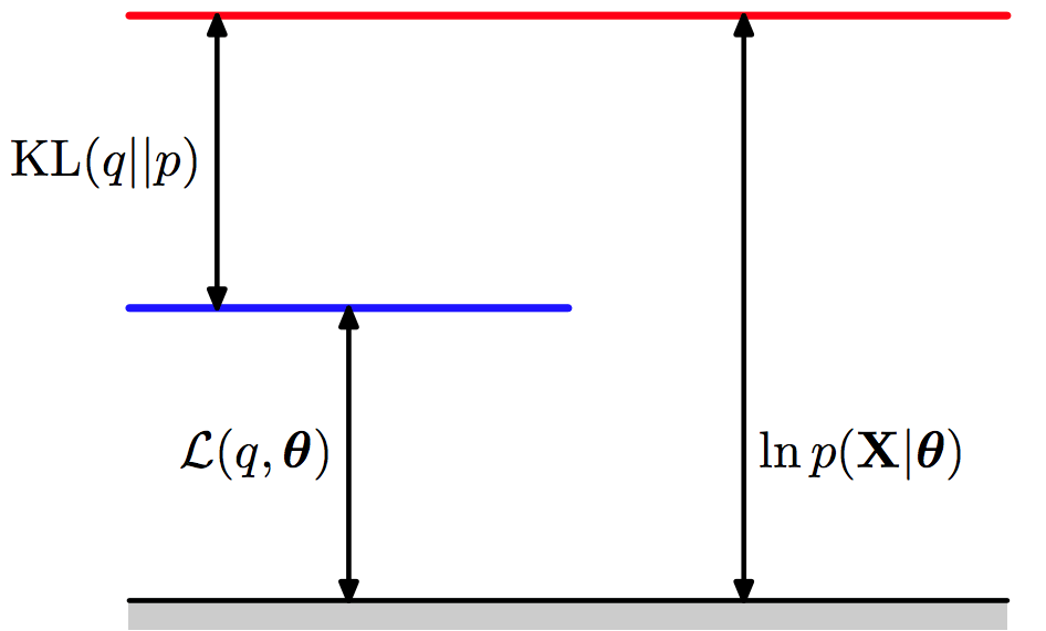
因为KL散度是非负的,所以$\ln p(x; \theta) \ge F(q, \theta)$,所以ELBO给marginal likelihood提供了下限。所以Expectation Maximization (EM)和variational inference最大化variational lower bound,而不直接最大化marginal likelihood
假设我们能analytically得到 $p(z | x; \theta^{OLD})$(对高斯混合模型来说就是softmax),那我们就能$q(z) = p(z | x; \theta^{OLD})$
$$\begin{aligned} F(q, \theta) & = \int q(z) \ln \Big( \frac{p(x, z; \theta)}{q(z)} \Big) dz \\ & = \int q(z) \ln p(x, z; \theta) dz - \int q(z) \ln q(z) dz \\ & = \int p(z | x; \theta^{OLD}) \ln p(x, z; \theta) dz \\ & \quad - \int p(z | x; \theta^{OLD}) \ln p(z | x; \theta^{OLD}) dz \\ & = Q(\theta, \theta^{OLD}) + H(q) \end{aligned}$$
第二项$H(z|x)$是给定x条件下z的熵,是$\theta^{OLD}$的函数,$\theta^{OLD}$当成已知项,所以这项是常数
EM算法的目标就是$\argmax\limits_\theta Q(\theta, \theta^{OLD})$
(Gibbs entropy)
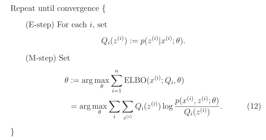
- E:计算$p(z | x; \theta^{OLD})$
- M:计算$\argmax\limits_\theta\displaystyle\int p(z | x; \theta^{OLD}) \ln p(x, z; \theta) dz$
> For example, the EM for the Gaussian Mixture Model consists of an expectation step where you compute the soft assignment of each datum to K clusters, and a maximization step which computes the parameters of each cluster using the assignment. However, for complex models, we cannot use the EM algorithm.
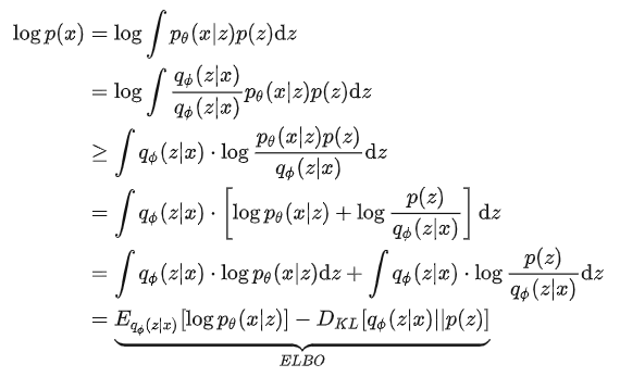
**另一种推导出ELBO的方法**,利用琴生不等式(函数是$\log x$):
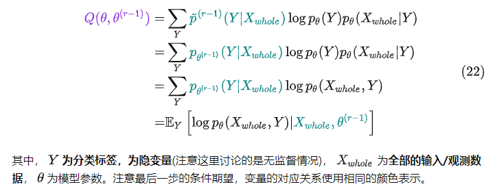
## 6.2 EM算法的训练流程
使用KL散度作为联合分布的差异性度量,然后对KL散度交替最小化
输入:观测变量数据X,隐变量数据Y,联合分布$p_\theta(X,Y)$,条件分布$p_\theta(Y|X)$<font color='green'>(总之是指含有未知数$\theta$的式子)</font>
输出:模型参数$\theta$
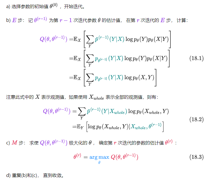
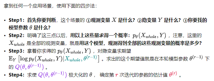
我的理解:
1. 先确定X,Y,θ
2. 给出Q关于θ的表达式
3. 重复步骤:代入θ计算E(Q),计算使E极大的θ
(EM算法的收敛性证明略)
