

在经典机器学习中,随机森林一直是一种灵丹妙药类型的模型。
该模型很棒有几个原因:
- 与许多其他算法相比,需要较少的数据预处理,因此易于设置
- 充当分类或回归模型
- 不太容易过度拟合
- 可以轻松计算特征重要性
在本文中,我想更好地理解构成随机森林的组件。为实现这一点,我将把随机森林解构为最基本的组成部分,并解释每个计算级别中发生的事情。到最后,我们将对随机森林的工作原理以及如何更直观地使用它们有更深入的了解。我们将使用的示例将侧重于分类,但许多原则也适用于回归场景。
1. 运行随机森林
让我们从调用经典的随机森林模式开始。这是最高级别,也是许多人在用 Python 训练随机森林时所做的。
如果我想运行随机森林来预测我的目标列,我只需执行以下操作
from sklearn.ensemble import RandomForestClassifier
from sklearn.model_selection import train_test_split

X_train, X_test, y_train, y_test = train_test_split(df.drop('target', axis=1), df['target'], test_size=0.2, random_state=0)

# Train and score Random Forest
simple_rf_model = RandomForestClassifier(n_estimators=100, random_state=0)
simple_rf_model.fit(X_train, y_train)
print(f"accuracy: {simple_rf_model.score(X_test, y_test)}")

# accuracy: 0.93
运行随机森林分类器非常简单。我刚刚定义了 n_estimators 参数并将 random_state 设置为 0。我可以根据个人经验告诉你,很多人只会看着那个 .93 ,很高兴,然后在野外部署那个东西。
simple_rf_model = RandomForestClassifier(n_estimators=100, random_state=0)
随机状态是大多数数据科学模型的一个特征,它确保其他人可以重现你的工作。我们不会太担心那个参数。
让我们深入了解一下 n_estimators。如果我们看一下 scikit-learn 文档,定义是这样的:
森林中树木的数量。
2. 调查树木的数量
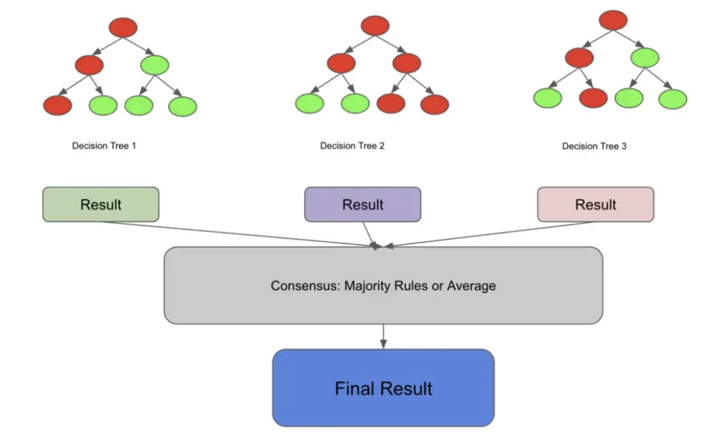
在这一点上,让我们更具体地定义随机森林。随机森林是一种集成模型,它是许多决策树的共识。该定义可能不完整,但我们会回来讨论它。
这可能会让您认为,如果将其分解为如下内容,您可能会得到一个随机森林:
# Create decision trees
tree1 = DecisionTreeClassifier().fit(X_train, y_train)
tree2 = DecisionTreeClassifier().fit(X_train, y_train)
tree3 = DecisionTreeClassifier().fit(X_train, y_train)

# predict each decision tree on X_test
predictions_1 = tree1.predict(X_test)
predictions_2 = tree2.predict(X_test)
predictions_3 = tree3.predict(X_test)
print(predictions_1, predictions_2, predictions_3)

# take the majority rules
final_prediction = np.array([np.round((predictions_1[i] + predictions_2[i] + predictions_3[i])/3) for i in range(len(predictions_1))])
print(final_prediction)
在上面的例子中,我们在 X_train 上训练了 3 棵决策树,这意味着 n_estimators = 3。在训练完这 3 棵树之后,我们在同一测试集上预测每棵树,然后最终采用 3 棵树中的 2 棵树进行预测。
有点道理,但这看起来并不完全正确。如果所有的决策树都在相同的数据上进行训练,它们会不会大多得出相同的结论,从而否定集成的优势?
3. 置换抽样
让我们在之前的定义中添加一个词:随机森林是一种集成模型,它是许多不相关决策树的共识。
决策树可以通过两种方式变得不相关:
- 您有足够大的数据集大小,您可以在其中将数据的独特部分采样到每个决策树。这不是很流行,而且通常需要大量数据。
- 您可以利用一种称为替换采样的技术。有放回抽样意味着从总体中抽取的样本在抽取下一个样本之前返回到总体中。
为了解释有放回抽样,假设我有 5 个弹珠和 3 种颜色,所以我的总体看起来像这样:
blue, blue, red, green, red
如果我想采样一些弹珠,我通常会挑出一对,最后可能会是:
blue, red
这是因为一旦我捡起红色,我就没有把它放回原来的弹珠堆中。
但是,如果我进行有放回抽样,我实际上可以两次拿起我的任何弹珠。因为红色回到了我的筹码中,所以我有机会再次捡起它。
red, red
在随机森林中,默认构建的样本大约是原始种群大小的 2/3。如果我的原始训练数据是 1000 行,那么我提供给树的训练数据样本可能是 670 行左右。也就是说,在构建随机森林时尝试不同的采样率将是一个很好的调整参数。
与最后一个片段不同,下面的代码更接近 n_estimators = 3 的随机森林代码。
import numpy as np
import pandas as pd
from sklearn.tree import DecisionTreeClassifier
from sklearn.model_selection import train_test_split
# Take 3 samples with replacement from X_train for each tree
df_sample1 = df.sample(frac=.67, replace=True)
df_sample2 = df.sample(frac=.67, replace=True)
df_sample3 = df.sample(frac=.67, replace=True)
X_train_sample1, X_test_sample1, y_train_sample1, y_test_sample1 = train_test_split(df_sample1.drop('target', axis=1), df_sample1['target'], test_size=0.2)
X_train_sample2, X_test_sample2, y_train_sample2, y_test_sample2 = train_test_split(df_sample2.drop('target', axis=1), df_sample2['target'], test_size=0.2)
X_train_sample3, X_test_sample3, y_train_sample3, y_test_sample3 = train_test_split(df_sample3.drop('target', axis=1), df_sample3['target'], test_size=0.2)
# Create the decision trees
tree1 = DecisionTreeClassifier().fit(X_train_sample1, y_train_sample1)
tree2 = DecisionTreeClassifier().fit(X_train_sample2, y_train_sample2)
tree3 = DecisionTreeClassifier().fit(X_train_sample3, y_train_sample3)
# predict each decision tree on X_test
predictions_1 = tree1.predict(X_test)
predictions_2 = tree2.predict(X_test)
predictions_3 = tree3.predict(X_test)
df = pd.DataFrame([predictions_1, predictions_2, predictions_3]).T
df.columns = ["tree1", "tree2", "tree3"]
# take the majority rules
final_prediction = np.array([np.round((predictions_1[i] + predictions_2[i] + predictions_3[i])/3) for i in range(len(predictions_1))])
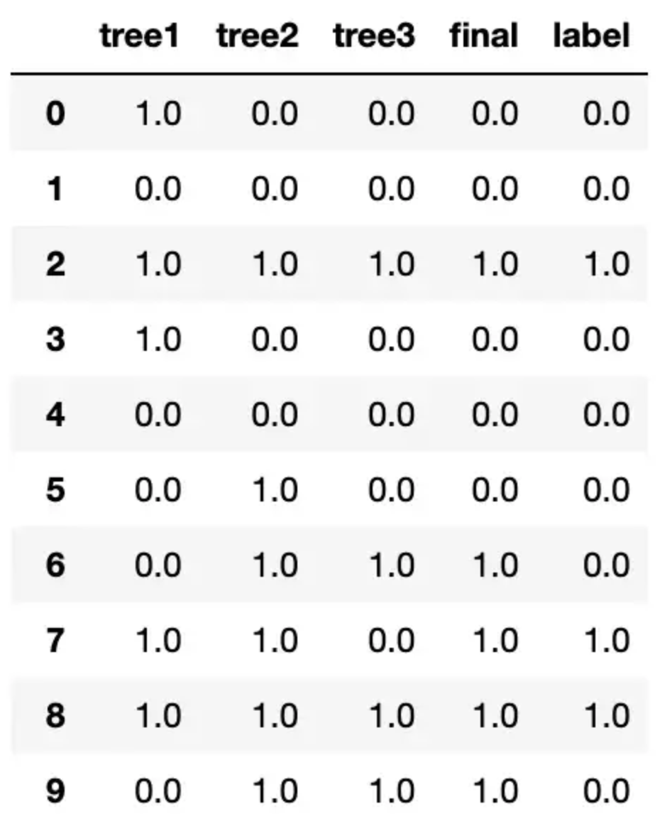
preds = pd.DataFrame([predictions_1, predictions_2, predictions_3, final_prediction, y_test]).T.head(20)
preds.columns = ["tree1", "tree2", "tree3", "final", "label"]
preds
4. 装袋分类器
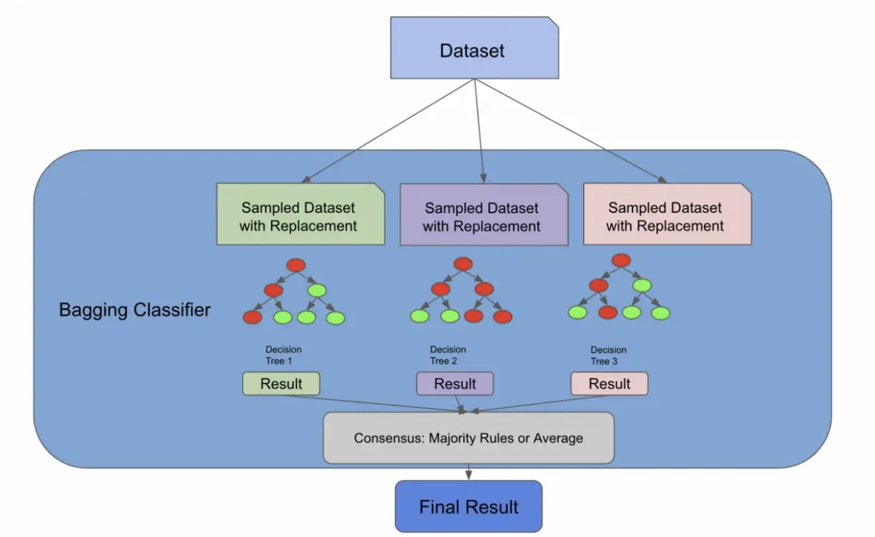
我们将在此时引入一种称为引导聚合的新算法,也称为装袋,但请放心,这将与随机森林相关联。我们引入这个新概念的原因是因为正如我们在下图中所看到的,到目前为止我们所做的一切实际上都是 BaggingClassifier 所做的!
在下面的代码中,BaggingClassifier 有一个名为 bootstrap 的参数,它实际上执行了我们刚刚手动执行的带替换采样步骤。 sklearn 随机森林实现也存在相同的参数。如果 bootstrapping 为假,我们将为每个分类器使用整个群体。
import numpy as np
from sklearn.tree import DecisionTreeClassifier
from sklearn.ensemble import BaggingClassifier

# Number of trees to use in the ensemble
n_estimators = 3

# Initialize the bagging classifier
bag_clf = BaggingClassifier(
    DecisionTreeClassifier(), n_estimators=n_estimators, bootstrap=True)

# Fit the bagging classifier on the training data
bag_clf.fit(X_train, y_train)

# Make predictions on the test data
y_pred = bag_clf.predict(X_test)
pd.DataFrame([y_pred, y_test]).T
BaggingClassifiers 很棒,因为您可以将它们与未命名为决策树的估算器一起使用!您可以插入许多算法,然后 Bagging 将其变成一个集成解决方案。随机森林算法实际上扩展了装袋算法(如果 bootstrapping = true),因为它部分利用装袋来形成不相关的决策树。
然而,即使 bootstrapping = false,随机森林也会多走一步以真正确保树不相关——特征采样。
5. 特征采样
特征抽样意味着不仅对行进行抽样,对列也进行抽样。与行不同,随机森林的列是在没有替换的情况下进行采样的,这意味着我们不会有重复的列来训练 1 棵树。
有很多方法可以对特征进行采样。您可以指定要采样的固定最大特征数,取特征总数的平方根,或尝试使用日志。这些方法中的每一种都有权衡取舍,并且将取决于您的数据和用例。
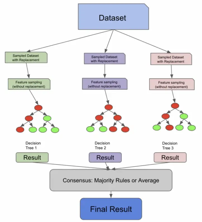
下面的代码片段使用 sqrt 技术对列进行采样,对行进行采样,训练 3 个决策树,并使用多数规则进行预测。我们首先执行替换采样,他们对列进行采样,训练我们的个体树,让我们的树对我们的测试数据进行预测,然后采用多数规则共识。
import numpy as np
import pandas as pd
import math
from sklearn.tree import DecisionTreeClassifier
from sklearn.model_selection import train_test_split

# take 3 samples from X_train for each tree
df_sample1 = df.sample(frac=.67, replace=True)
df_sample2 = df.sample(frac=.67, replace=True)
df_sample3 = df.sample(frac=.67, replace=True)

# split off train set
X_train_sample1, y_train_sample1 = df_sample1.drop('target', axis=1), df_sample1['target']
X_train_sample2, y_train_sample2 = df_sample2.drop('target', axis=1), df_sample2['target']
X_train_sample3, y_train_sample3 = df_sample3.drop('target', axis=1), df_sample3['target']

# get sampled features for train and test using sqrt, note how replace=False now
num_features = len(X_train.columns)
X_train_sample1 = X_train_sample1.sample(n=int(math.sqrt(num_features)), replace=False, axis = 1)
X_train_sample2 = X_train_sample2.sample(n=int(math.sqrt(num_features)), replace=False, axis = 1)
X_train_sample3 = X_train_sample3.sample(n=int(math.sqrt(num_features)), replace=False, axis = 1)

# create the decision trees, this time we are sampling columns
tree1 = DecisionTreeClassifier().fit(X_train_sample1, y_train_sample1)
tree2 = DecisionTreeClassifier().fit(X_train_sample2, y_train_sample2)
tree3 = DecisionTreeClassifier().fit(X_train_sample3, y_train_sample3)

# predict each decision tree on X_test
predictions_1 = tree1.predict(X_test[X_train_sample1.columns])
predictions_2 = tree2.predict(X_test[X_train_sample2.columns])
predictions_3 = tree3.predict(X_test[X_train_sample3.columns])
preds = pd.DataFrame([predictions_1, predictions_2, predictions_3]).T
preds.columns = ["tree1", "tree2", "tree3"]

# take the majority rules
final_prediction = np.array([np.round((predictions_1[i] + predictions_2[i] + predictions_3[i])/3) for i in range(len(predictions_1))])
preds = pd.DataFrame([predictions_1, predictions_2, predictions_3, final_prediction, y_test]).T.head(20)
preds.columns = ["tree1", "tree2", "tree3", "final", "label"]
当我运行这段代码时,我发现我的决策树开始预测不同的事情,这表明我们已经删除了树之间的很多相关性。
6. 决策树基础
到目前为止,我们已经解构了数据是如何输入到大量决策树中的。在前面的代码示例中,我们使用了 DecisionTreeClassifier() 来训练决策树,但我们需要解构决策树才能完全理解随机森林。
决策树,顾名思义,看起来像一棵倒置的树。在高层次上,该算法试图提出问题以将数据拆分到不同的节点。下图显示了决策树的外观示例。
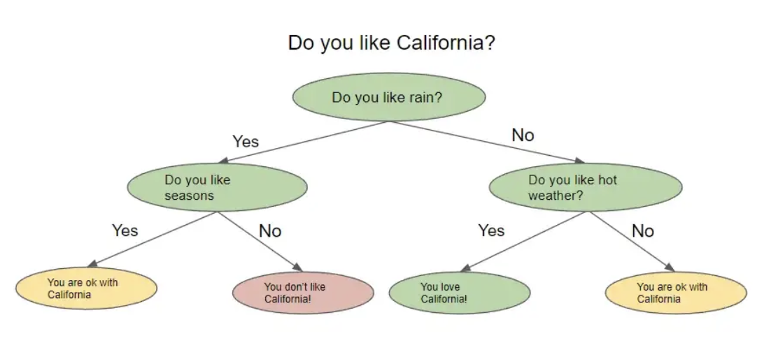
决策树根据前一个问题的答案提出一系列问题。对于它提出的每个问题,都可能有多个答案,我们将其可视化为拆分节点。上一个问题的答案将决定树将要问的下一个问题。在问了一系列问题后的某个时候,您会得出答案。
但是你怎么知道你的答案是准确的,或者你问了正确的问题呢?您实际上可以用几种不同的方式评估您的决策树,我们当然也会分解这些方法。
7. 熵和信息增益
在这一点上,我们需要讨论一个叫做熵的新术语。在高层次上,熵是衡量节点中不纯程度或随机性水平的一种方法。顺便说一句,还有另一种流行的方法来衡量节点的不纯度,称为基尼不纯度,但我们不会在这篇文章中解构该方法,因为它与许多关于熵的概念重叠,尽管计算略有不同。一般的想法是熵或基尼杂质越高,节点中的方差越大,我们的目标是减少这种不确定性。
决策树试图通过将它们询问的节点分成更小的更同质的节点来最小化熵。熵的实际公式是

为了分解熵,让我们回到那个弹珠的例子:
假设我有 10 个弹珠。其中5个是蓝色的,5个是绿色的。我的集体数据集的熵为 1.0,计算熵的代码如下:
from collections import Counter
from math import log2

# my predictor classes are 0 or 1. 0 is a blue marble, 1 is a green marble.
data = [0, 0, 0, 1, 1, 1, 1, 0, 1, 0]
# get length of labels
len_labels = len(data)
def calculate_entropy(data, len_labels):
    # we do a count of each class
    counts = Counter(labels)
    # we calculate the fractions, the output should be [.5, .5] for this example
    probs = [count / num_labels for count in counts.values()]
    # the actual entropy calculation
    return - sum(p * log2(p) for p in probs)

calculate_entropy(labels, num_labels)
如果数据完全被绿色弹珠填满,则熵将为 0,并且越接近 50% 的分割,熵就会增加。
每次我们减少熵时,我们都会获得一些关于数据集的信息,因为我们已经减少了随机性。信息增益告诉我们哪个特征相对允许我们最好地最小化我们的熵。计算信息增益的方法是:
entropy(parent) — [weighted_average_of_entropy(children)]
在这种情况下,父节点是原始节点,子节点是拆分节点的结果。
为了计算信息增益,我们执行以下操作:
- 计算父节点的熵
- 将父节点拆分为子节点
- 为每个子节点创建权重。这是由 number_of_samples_in_child_node / number_of_samples_in_parent_node 测量的
- 计算每个子节点的熵
- 通过计算 weightentropy_of_child1 + weightentropy_of_child2 创建 [weighted_average_of_entropy(children)]
- 从父节点的熵中减去这个加权熵
下面的代码为一个父节点被拆分为 2 个子节点实现了一个简单的信息增益
def information_gain(left_labels, right_labels, parent_entropy):
    """Calculate the information gain of a split"""
    # calculate the weight of the left node
    proportion_left_node = float(len(left_labels)) / (len(left_labels) + len(right_labels))
    #calculate the weight of the right node
    proportion_right_node = 1 - proportion_left_node
    # compute the weighted average of the child node
    weighted_average_of_child_nodes = ((proportion_left_node * entropy(left_labels)) + (proportion_right_node * entropy(right_labels)))
    # return the parent node entropy - the weighted entropy of child nodes
    return parent_entropy - weighted_average_of_child_nodes
8. 解构决策树
考虑到这些概念,我们准备实现一个小的决策树!
在没有任何指导的情况下,决策树将不断分裂节点,直到所有最终叶节点都是纯节点。控制树的复杂性的想法称为剪枝,我们可以在树完全构建后剪枝,也可以在树的生长阶段之前用一定的参数预先剪枝。预剪枝树复杂性的一些方法是控制分裂的数量,限制最大深度(从根节点到叶节点的最长距离),或设置信息增益。
下面的代码将所有这些概念联系在一起
- 从一个数据集开始,您可以在其中预测目标变量
- 计算原始数据集(根节点)的熵(或基尼杂质)
- 查看每个特征并计算信息增益
- 选择具有最佳信息增益的最佳特征,这与导致熵减少最多的特征相同
- 继续增长直到满足我们的停止条件——在这种情况下,它是我们的最大深度限制和熵为 0 的节点。
import pandas as pd
import numpy as np
from math import log2

def entropy(data, target_col):
    # calculate the entropy of the entire dataset
    values, counts = np.unique(data[target_col], return_counts=True)
    entropy = np.sum([-count/len(data) * log2(count/len(data)) for count in counts])
    return entropy

def compute_information_gain(data, feature, target_col):
    parent_entropy = entropy(data, target_col)
    # calculate the information gain for splitting on a given feature
    split_values = np.unique(data[feature])
    # initialize at 0
    weighted_child_entropy = 0
    # compute the weighted entropy, remember that this is related to the number of points in the new node
    for value in split_values:
        sub_data = data[data[feature] == value]
        node_weight = len(sub_data)/len(data)
        weighted_child_entropy += node_weight * entropy(sub_data, target_col)
    # same calculation as before, we just subtract the weighted entropy from the parent node entropy
    return parent_entropy - weighted_child_entropy

def grow_tree(data, features, target_col, depth=0, max_depth=3):
    # we set a max depth of 3 to "pre-prune" or limit the tree complexity
    if depth >= max_depth or len(np.unique(data[target_col])) == 1:
        # stop growing the tree if maximum depth is reached or all labels are the same. All labels being the same means the entropy is 0
        return np.unique(data[target_col])[0]
    # we compute the best feature (or best question to ask) based on information gain
    node = {}
    gains = [compute_information_gain(data, feature, target_col) for feature in features]
    best_feature = features[np.argmax(gains)]

    for value in np.unique(data[best_feature]):
        sub_data = data[data[best_feature] == value]
        node[value] = grow_tree(sub_data, features, target_col, depth+1, max_depth)

    return node


# simulate some data and make a dataframe, note how we have a target
data = {
    'A': [1, 2, 1, 2, 1, 2, 1, 2],
    'B': [3, 3, 4, 4, 3, 3, 4, 4],
    'C': [5, 5, 5, 5, 6, 6, 6, 6],
    'target': [0, 0, 0, 1, 1, 1, 1, 0]
}
df = pd.DataFrame(data)

# define our features and label
features = ["A", "B", "C"]
target_col = "target"

# grow the tree
tree = grow_tree(df, features, target_col, max_depth=3)
print(tree)
在这棵树上进行预测意味着用新数据遍历生长的树,直到它到达叶节点。最后的叶节点是预测。
总结
总结一下我们学到的东西:
- 随机森林实际上是一组不相关的决策树进行预测并达成共识。这种共识是回归问题的平均分数和分类问题的多数规则
- 随机森林通过利用装袋和特征采样来减轻相关性。通过利用这两种技术,各个决策树正在查看我们集合的特定维度并根据不同因素进行预测。
- 通过在产生最高信息增益的特征上拆分数据来生成决策树。信息增益被测量为杂质的最高减少。杂质通常通过熵或基尼杂质来衡量。
- 随机森林能够通过特征重要性实现有限水平的可解释性,特征重要性是特征的平均信息增益的度量。
- 随机森林还能够在训练时进行某种形式的交叉验证,这是一种称为 OOB 错误的独特技术。这是可能的,因为算法对上游数据进行采样的方式。
本文由mdnice多平台发布
