

“开启掘金成长之旅!这是我参与「掘金日新计划 · 2 月更文挑战」的第 1 天,点击查看活动详情”
本文仅作为学习参考文章第二节关于线性单元和梯度下降的一个补充,主要是代码部分python画图从python2改到python3,无其他改动
关于梯度下降和反向传播之前的博文已经写过,此处不再详述
参考资料:www.zybuluo.com/hanbingtao/…
关于个人对于梯度下降以及反向传播的理解:blog.csdn.net/Lian_Ge_Blo…
#!/usr/bin/env python
# -*- coding: UTF-8 -*-

# 其实代码同参考文章作者所说,只不过是去掉了激活函数,也就是分类的过程,其他并无任何区别,多了画图部分也只是方便理解。
from perceptron import Perceptron

# 定义激活函数f
f = lambda x: x


class LinearUnit(Perceptron):
    def __init__(self, input_num):
        '''初始化线性单元,设置输入参数的个数'''
        Perceptron.__init__(self, input_num, f)


def get_training_dataset():
    '''
    捏造5个人的收入数据
    '''
    # 构建训练数据
    # 输入向量列表,每一项是工作年限
    input_vecs = [[5], [3], [8], [1.4], [10.1]]
    # 期望的输出列表,月薪,注意要与输入一一对应
    labels = [5500, 2300, 7600, 1800, 11400]
    return input_vecs, labels


def train_linear_unit():
    '''
    使用数据训练线性单元
    '''
    # 创建感知器,输入参数的特征数为1(工作年限)
    lu = LinearUnit(1)
    # 训练,迭代10轮, 学习速率为0.01
    input_vecs, labels = get_training_dataset()
    lu.train(input_vecs, labels, 10, 0.01)
    # 返回训练好的线性单元
    return lu


def plot(linear_unit):
    import matplotlib.pyplot as plt
    input_vecs, labels = get_training_dataset()
    fig = plt.figure()
    # 分区域,111表示第一行第一列的第一个区域
    ax = fig.add_subplot(111)
    # scatter 散点图
    ax.scatter(list(map(lambda x: x[0], input_vecs)), labels)
    weights = linear_unit.weights
    bias = linear_unit.bias
    x = range(0,12,1)
    y = list(map(lambda x:weights[0] * x + bias, x))
    ax.plot(x, y)
    plt.show()


if __name__ == '__main__':
    '''训练线性单元'''
    linear_unit = train_linear_unit()
    # 打印训练获得的权重
    print(linear_unit)
    # 测试
    print('Work 3.4 years, monthly salary = %.2f' % linear_unit.predict([3.4]))
    print('Work 15 years, monthly salary = %.2f' % linear_unit.predict([15]))
    print('Work 1.5 years, monthly salary = %.2f' % linear_unit.predict([1.5]))
    print('Work 6.3 years, monthly salary = %.2f' % linear_unit.predict([6.3]))
    plot(linear_unit)
代码运行结果和图示分别为:(见链接):(深度学习2 --线性单元和梯度下降_Lian_Ge_Blog的博客-CSDN博客)
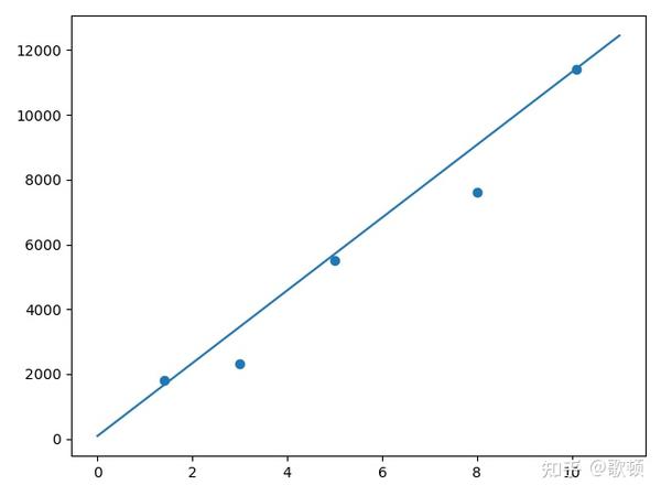
折线图
