本文已参与「新人创作礼」活动,一起开启掘金创作之路。
本文首发于CSDN。
诸神缄默不语-个人CSDN博文目录
Combining Label Propagation and Simple Models Out-performs Graph Neural Networks
@[toc]
1. 模型构造思路
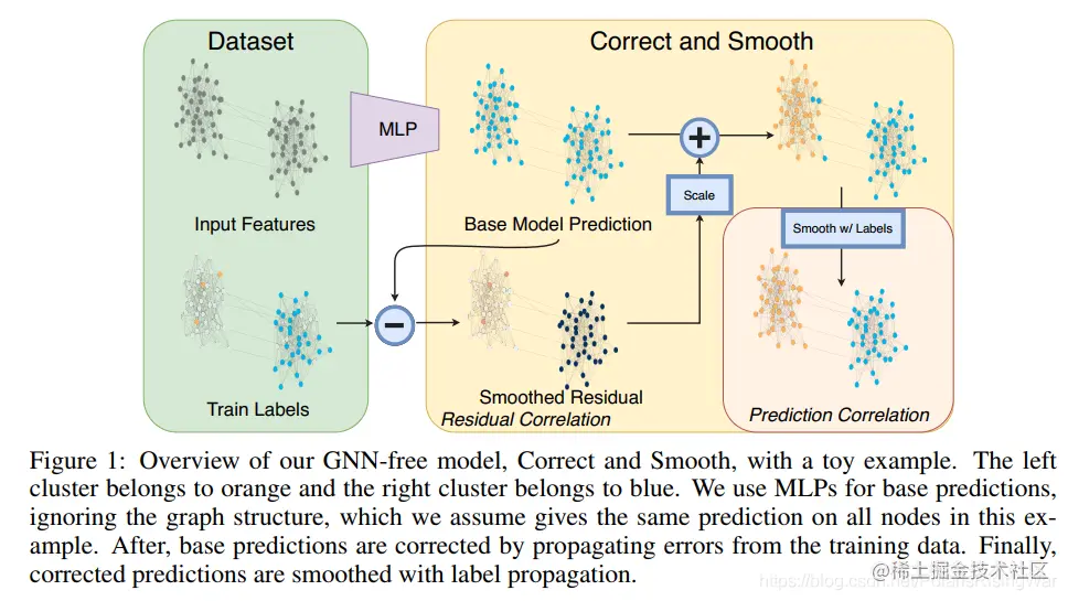
本文的核心是将GNN模型给解耦了。
大概思路是 predictor → correct:平滑error → smooth:平滑标签
平滑的思路很像APPNP那篇。那篇我也写了笔记,可资参考:Re0:读论文 PPNP/APPNP Predict then Propagate: Graph Neural Networks meet Personalized PageRank
predictor可以用任一预测模型,所以这个模型也可以结合到别的GNN模型上。
别的,因为我没咋看懂这篇论文,所以不多赘述。
这篇论文原理上我主要有两大迷惑:
-
它这个correct阶段跑的是这个很类似于PPR的迭代模型:E(t+1)=(1−α)E+αSE(t)(E 是残差)
就PPR的稳定状态见APPNP,就是PPNP那形式嘛。
然后说这个模型最后会迭代到这个目标函数上:E^=argmintrace (WT(I−S)W)+µ∣∣W−E∣∣F2
为啥啊?????
我看了一下论文里引用了 Dengyong Zhou, Olivier Bousquet, Thomas N Lal, Jason Weston, and Bernhard Scholkopf. Learning with local and global consistency. In Advances in neural information processing systems, pp. 321–328, 2004. 这篇论文,但是这篇我更看不懂了……
所以这个迭代公式是怎么收敛到目标函数的啊?论文里还说 I−S 是误差估计在全图上的平滑,在这部分我也没有搞懂?
-
还有就是这个误差模长会随迭代而越来越小?
这个公式我也没想明白是怎么推导得来的:∣∣E(t+1)∣∣2≤(1−α)∣∣E∣∣+α∣∣S∣∣2∣∣E(t)∣∣2=(1−α)∣∣E∣∣2+α∣∣E(t)∣∣2
总之没有搞懂。具体不赘,有缘再补。
2. Notation和模型介绍
2.1 notation
\text{无标签节点}\ &U
\\ \text{有标签节点}\ &L
\\ \text{training set}\ &L_t
\\ \text{validation set}\ &L_v
\\ \text{normalized adjacency matrix}\ &S=\mathbf{D}^{-\frac{1}{2}}\mathbf{A}\mathbf{D}^{-\frac{1}{2}}
\\ \text{prediction}\ &Z\in\mathbb{R}^{n\times c}
\\ \text{error matrix}\ &E\in\mathbb{R}^{n\times c}
\end{aligned}$$
未完待续。
## 2.2 模型介绍
<font color='red'>我觉得模型有问题,以下我的理解都标色了</font>
predictor + post-processing
不是端到端的训练,也就是说correct+smooth是不跟predictor一起train的。就C&S阶段就是直接加上去的。
不像APPNP,propagate阶段是跟着predict一起train的,是端到端的。
### 2.2.1 Predictor
首先在图上应用一个仅使用节点特征的预测模型。
在本文中选用一个线性模型或浅MLP,应用softmax。损失函数为交叉熵。
得到base prediction $Z\in\mathbb{R}^{n\times c}$
### 2.2.2 Correct阶段
定义error matrix $E\in\mathbb{R}^{n\times c}$:误差是训练集上的残差,其他split上为0
$E_{L_t} = Z_{L_t} − Y_{L_t},\ E_{L_v} = 0,\ E_U = 0$
迭代:$E^{(t+1) }= (1 − α)E + αSE^{(t)}$(其中 $E^{(0)}=E$ )
平滑误差:$Z^{(r)} = Z + \hat{E}$
<font color='red'>这里应该是减号,我的实验结果证明了这一结果。就E=Z-Y的话那就应该Z-E才能靠近Y,所以改成减号才比较合理嘛。
要么就是上上句公式Z和Y写反了,那就是E=Y-Z,所以平滑误差时Z+E才合理(PyG的实现是改了这部分。其实改这边更合理,因为残差本来就是 $y-\hat{y}$ 真实值减拟合值 嘛)
C&S官方实现里也是E=Y-Z,然后Z+=E这样写的:代码截图自[CorrectAndSmooth/outcome_correlation.py at master · CUAI/CorrectAndSmooth](https://github.com/CUAI/CorrectAndSmooth/blob/master/outcome_correlation.py)(这个代码写得还是,不知道怎么形容,反正看多了各种作者写的代码后,我现在觉得PyG的代码都算比较好懂的了。所以我看到PTA那种代码的时候我都被其之简洁明确而惊诧甚矣了好吗!!!)


</font>
<font color='orange'>(跟学长讨论了一下,感觉这个比较像DNN里面的梯度更新)</font>
scale残差的两种方法:
1. Autoscale
$e_j\in\mathbb{R}^c$ 为 $E$ 的第 $j$ 行
$σ =\dfrac{1}{|L_t|}\sum_{j\in L_t}||e_j||_1$
对无标签节点的corrected prediction:$Z^{(r)}_{i,:}=Z_{i,:}+σ\hat{E}_{:,i}/||\hat{E}_{:,i}^T||_1$
2. Scaled Fixed Diffusion (FDiff-scale)
迭代 $E^{(t+1)}_U = [D^{−1}AE^{(t)}]_U$(<font color='red'>我代码里还是用的S。应该是都行的,这个看我写的APPNP那篇笔记吧,有讲这两个矩阵是咋回事</font>),固定 $E_L^{(t)} = E_L$ 直至趋近于 $\hat{E}$(起始状态:$E^{(0)}=E$ )
设置超参 $s$:$Z^{(r)} = Z + s\hat{E}$
### 2.2.3 Smooth阶段
定义best guess $G\in\mathbb{R}^{n×c}$ of the labels:
$$G_{L_t} = Y_{L_t},\ G_{L_v,U} = Z_{L(v),U}^{(r)}$$
(验证集数据也可以用其真实值,见实验设置)
<br>
迭代:$G^{(t+1) }= (1 − α)G + αSG^{(t)}$(其中 $G^{(0)}=G$ )
直至收敛,得到最终预测结果 $\hat{Y}$
对无标签节点 $i\in U$ 的最终预测标签就是 $\argmax_{j\in\{1,...c\}}\hat{Y}_{ij}$
# 3. 详细的数学推导和证明
还没看,待补。
# 4. 实验结果
还没看,待补。
# 5. 代码实现和复现
## 5.1 论文官方实现
[CUAI/CorrectAndSmooth: [ICLR 2021] Combining Label Propagation and Simple Models Out-performs Graph Neural Networks (https://arxiv.org/abs/2010.13993)](https://github.com/CUAI/CorrectAndSmooth)
讲解待补。
## 5.2 PyG官方实现
[CorrectAndSmooth类官方文档](https://pytorch-geometric.readthedocs.io/en/latest/_modules/torch_geometric/nn/models/correct_and_smooth.html#CorrectAndSmooth)
源代码:[torch_geometric.nn.models.correct_and_smooth — pytorch_geometric 1.7.2 documentation](https://pytorch-geometric.readthedocs.io/en/latest/_modules/torch_geometric/nn/models/correct_and_smooth.html)
作为卷都卷不动的post-processing模型,终于不用MessagePassing而正常用torch.nn.Module基类了。这是什么值得开心的事情吗?值得个屁,这个模型用了LabelPropagation类……
呀咩咯,我受够了看PyG这个大佬作者虽然很牛逼但是没有注释而且严重依赖他自己写的其他没有注释但是很牛逼的包的源码了,放过我吧!
所以还没看,待补。
## 5.3 我自己写的复现
```python
def edge_index2sparse_tensor(edge_index,node_num):
sizes=(node_num,node_num)
v=torch.ones(edge_index[0].numel()).to(hp['device']) #边数
return torch.sparse_coo_tensor(edge_index, v, sizes)
class CNS_self(torch.nn.Module):
#参数照抄PyG了,意思也一样
def __init__(self,correct_layer,correct_alpha,smooth_layer,smooth_alpha,autoscale,scale):
super(CNS_self,self).__init__()
self.correct_layer=correct_layer
self.correct_alpha=correct_alpha
self.smooth_layer=smooth_layer
self.smooth_alpha=smooth_alpha
self.autoscale=autoscale
self.scale=scale
def correct(self,Z,Y,mask,edge_index):
"""
Z:base prediction
Y:true label(第一维尺寸是训练集节点数)
mask:训练集mask
"""
#将Y扩展为独热编码矩阵
Y=F.one_hot(Y)
num_nodes=Z.size()[0]
num_features=Z.size()[1]
E=torch.zeros(num_nodes,num_features).to(hp['device'])
E[mask]=Z[mask]-Y
edge_index, _ = pyg_utils.add_self_loops(edge_index,num_nodes=num_nodes) #添加自环(\slide{A})
adj=edge_index2sparse_tensor(edge_index,num_nodes)
degree_vector=torch.sparse.sum(adj,0) #度数向量
degree_vector=degree_vector.to_dense().cpu()
degree_vector=np.power(degree_vector,-0.5)
degree_matrix=torch.diag(degree_vector).to(hp['device'])
adj=torch.sparse.mm(adj.t(),degree_matrix.t())
adj=adj.t()
adj=torch.mm(adj,degree_matrix)
adj=adj.to_sparse()
x=E.clone()
if self.autoscale==True:
for k in range(self.correct_layer):
x=torch.sparse.mm(adj,x)
x=x*self.correct_alpha
x=x+(1-self.correct_alpha)*E
sigma=1/(mask.sum().item())*(E.sum())
Z=Z-x
Z[~mask]=Z[~mask]-sigma*F.softmax(x[~mask],dim=1)
else:
for k in range(self.correct_layer):
x=torch.sparse.mm(adj,x)
x=x*self.correct_alpha
x=x+(1-self.correct_alpha)*E
x[mask]=E[mask]
Z=Z-self.scale*x
return Z
def smooth(self,Z,Y,mask,edge_index):
#将Y扩展为独热编码矩阵
Y=F.one_hot(Y)
num_nodes=Z.size()[0]
G=Z.clone()
G[mask]=Y.float()
edge_index, _ = pyg_utils.add_self_loops(edge_index,num_nodes=num_nodes) #添加自环(\slide{A})
adj=edge_index2sparse_tensor(edge_index,num_nodes)
degree_vector=torch.sparse.sum(adj,0) #度数向量
degree_vector=degree_vector.to_dense().cpu()
degree_vector=np.power(degree_vector,-0.5)
degree_matrix=torch.diag(degree_vector).to(hp['device'])
adj=torch.sparse.mm(adj.t(),degree_matrix.t())
adj=adj.t()
adj=torch.mm(adj,degree_matrix)
adj=adj.to_sparse() #adj就是S
x=G.clone()
for k in range(self.smooth_layer):
x=torch.sparse.mm(adj,x)
x=x*self.smooth_alpha
x=x+(1-self.smooth_alpha)*G
return x
```
## 5.4 复现实验结果对比
我他妈的,我在一次非常粗糙的实验之中超过了PyG的官方实现!
但是懒得详细验证了。论文官方实现我看都没求看懂,去他妈的吧。
未完待续。
详见:[APPNP和C&S复现](https://github.com/PolarisRisingWar/all-notes-in-one/blob/main/APPNP%E5%92%8CC%26S%E5%A4%8D%E7%8E%B0.ipynb)
# 6. 参考资料
1. 本篇论文的讲解文章
1. [训练时间和参数量百倍降低,直接使用标签进行预测,性能竟超GNN](https://baijiahao.baidu.com/s?id=1682324318883133888&wfr=spider&for=pc)
3. [标签传播与简单模型结合可超越图神经网络 - 知乎](https://zhuanlan.zhihu.com/p/358074127)
4. [Combining Label Propagation and Simple Models OUT-PERFORMS Graph Networks_Milkha的博客-CSDN博客](https://blog.csdn.net/Miha_Singh/article/details/115242985)
这篇写 “*该论文针对GNN的解释性不足,GNN模型越来越大的问题,提出了“小米加步枪” — 用简单模型得到和GNN一样的水平。*” 感觉这种说法好好玩ww。
5. [文献阅读(40)ICLR2021-Combining Label Propagation and Simple Models Out-performs Graph Neural Networks_CSDNTianJi的博客-CSDN博客](https://blog.csdn.net/CSDNTianJi/article/details/114632230)
6. [C&S《Combining Label Propagation and Simple Models Out-performs Graph Neural Networks》理论与实战_智慧的旋风的博客-CSDN博客](https://blog.csdn.net/weixin_41650348/article/details/115301921)
7. [论文笔记:ICLR 2021 Combining Lable Propagation And Simple Models Out-Performs Graph Neural Network_饮冰l的博客-CSDN博客](https://blog.csdn.net/qq_44015059/article/details/113689870)
2. [矩阵的迹_百度百科](https://baike.baidu.com/item/%E7%9F%A9%E9%98%B5%E7%9A%84%E8%BF%B9/8889744?fr=aladdin)
4. Dengyong Zhou, Olivier Bousquet, Thomas N Lal, Jason Weston, and Bernhard Scholkopf. Learning with local and global consistency. In Advances in neural information processing systems, pp. 321–328, 2004.
妈的,完全看不懂,什么东西。
1. [Learning with Local and Global Consistency_何必浓墨重彩-CSDN博客](https://blog.csdn.net/wendox/article/details/50492131)
3. [Learning with local and global consistency阅读报告NIPS2003_不会讲段子的正能量小王子-CSDN博客](https://blog.csdn.net/u011070272/article/details/73606020)


