

开启掘金成长之旅!这是我参与「掘金日新计划 · 12 月更文挑战」的第4天
本文首发于CSDN。
诸神缄默不语-个人CSDN博文目录 cs224w(图机器学习)2021冬季课程学习笔记集合
@[toc]
YouTube 视频观看地址1 视频观看地址2 视频观看地址3 视频观看地址4
本章主要内容: 本章首先介绍了网络中社区community(或cluster / group)的概念,以及从社会学角度来证明了网络中社区结构的存在性。 接下来介绍了modularity概念衡量community识别效果。 然后介绍了Louvain算法[^8]识别网络中的community。 对于overlapping communiteis,本章介绍了BigCLAM[^14] 方法来进行识别。
1. Community Detection in Networks
- 图中的社区识别任务就是对节点进行聚类
- networks & communities
网络会长成图中这样:由多个内部紧密相连、互相只有很少的边连接的community组成。
- 从社会学角度理解这一结构:
在社交网络中,用户是被嵌入的节点,信息通过链接(长链接或短链接流动)。
以工作信息为例,Mark Granovetter 在其60年代的博士论文[^1] 中提出,人们通过人际交往来获知信息,但这些交际往往在熟人(长链接)而非密友(短链接)之间进行,也就是真找到工作的信息往往来自不太亲密的熟人。这与我们所知的常识相悖,因为我们可能以为好友之间会更容易互相帮助。
Granovetter认为友谊(链接)有两种角度: 一是structural视角,友谊横跨网络中的不同部分。 二是interpersonal视角,两人之间的友谊是强或弱的。
Granovetter在一条边的social和structural视角之间找到了联系:
- structure:structurally/well embeded / tightly-connected 的边也socially strong,长距离的、横跨社交网络不同部分的边则socially weak。 也就是community内部、紧凑的短边更strong,community之间、稀疏的长边更weak。
- information:长距离边可以使人获取网络中不同部分的信息,从而得到新工作。structurally embedded边在信息获取方面则是冗余的。
也就是说,你跟好友之间可能本来就有相近的信息源,而靠外面的熟人才可能获得更多新信息。
- triadic closure
triadic:三元; 三色系; 三色; 三重; 三合一;
community (tightly-connected cluster of nodes) 形成原因:如果两个节点拥有相同的邻居,那么它们之间也很可能有边。(如果网络中两个人拥有同一个朋友,那么它们也很可能成为朋友)
triadic closure = high clustering coefficient[^2] triadic closure产生原因:如果B和C拥有一个共同好友A,那么B更可能遇见C(因为他们都要和A见面),B和C会更信任彼此,A也有动机带B和C见面(因为要分别维持两段关系比较难),从而B和C也更容易成为好友。 Bearman和Moody的实证研究[^3] 证明,clustering coefficient低的青少年女性更容易具有自杀倾向。
- 多年来Granovetter的理论一直没有得到验证,但是我们现在有了大规模的真实交流数据(如email,短信,电话,Facebook等),从而可以衡量真实数据中的edge strength。
举例:数据集Onnela et al. 2007[^4] 20%欧盟国家人口的电话网络,以打电话的数量作为edge weight - edge overlap
两个节点 之间的edge overlap,是除本身节点之外,两个节点共同邻居占总邻居的比例:
overlap=0 时这条边是local bridge
当两个节点well-embeded或structurally strong时,overlap会较高。图中左上角overlap:0/6 图中右上角overlap:2/6 图中左下角overlap:4/6 图中右下角overlap:6/6
- 在电话网络[^4] 中,edge strength(电话数)和edge overlap之间具有正相关性:图中蓝色是真实数据,红色是重新排列edge strength之后的数据(对照组):
在真实图中,更embeded(密集)的部分edge strength也更高(红):
相比之下,strength被随机shuffle之后的结果就没有这种特性:
从strength更低的边开始去除,能更快disconnect网络(相当于把community之间的边去掉):
从overlap更低的边开始,disconnect更快:
- 从而,我们得到网络的概念图:由structurally embeded的很多部分组成,其内部链接更强,其之间链接更弱:
2. Network Communites
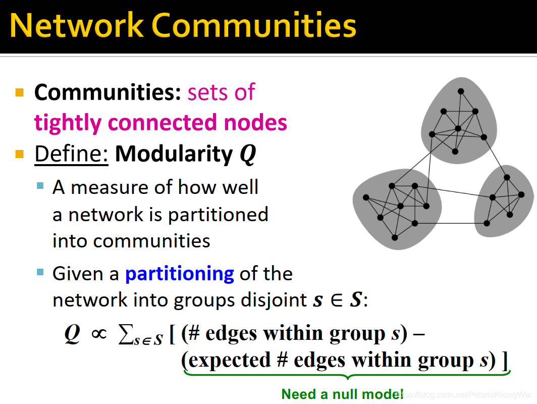
- network communites就是这些部分(也叫cluster,group,module):一系列节点,其内部有很多链接,与网络其他部分的外部链接很少
- 我们的目标就是给定一个网络,由算法自动找到网络中的communities(densely connected groups of nodes)
- 以Zachary’s Karate club network来说,通过社交关系创造的图就可以正确预判出成员冲突后会选择哪一边[^5]:
- 在付费搜索领域中,也可以通过社区识别来发现微众市场:举例来说,节点是advertiser和query/keyword,边是advertiser在该关键词上做广告。在赌博关键词中我们可以专门找到sporting betting这一小社区(微众市场):
- NCAA Football Network
节点是球队,边是一起打过比赛。通过社区识别算法也可以以较高的准确度将球队划分到不同的会议中:
- 定义modularity[^6] 衡量网络的一个社区划分partitioning(将节点划分到不同社区)的好坏程度:
已知一个划分,网络被划分到disjoint groups 中:
\\(\text{expected \# edges within group}\ s)\big]$$
其中expected # edges within group s需要一个null model
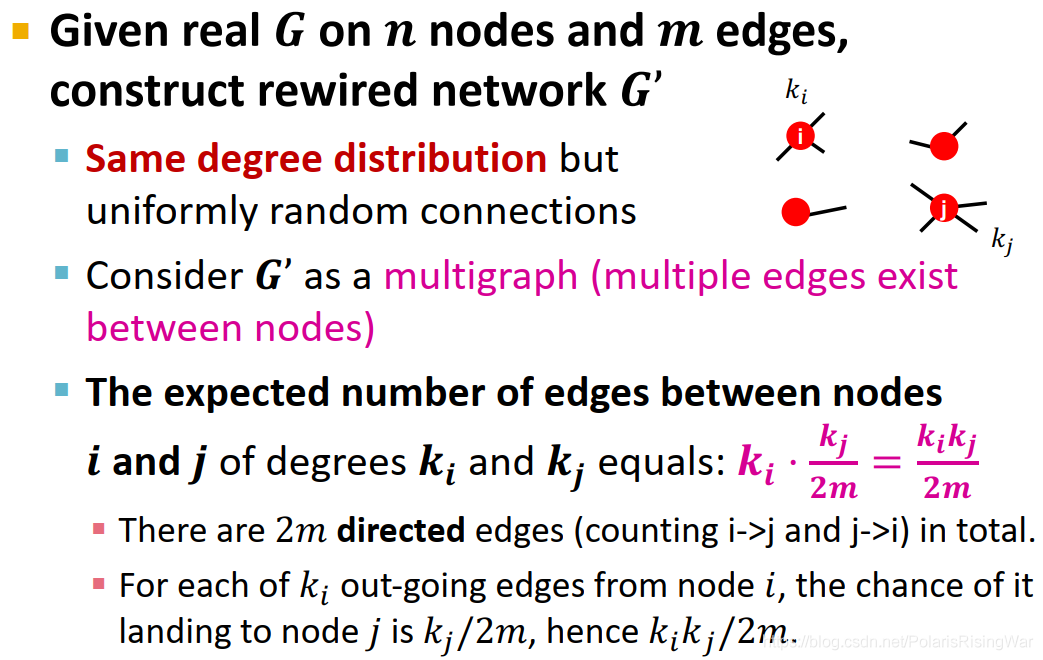
7. null model: configuration model[^7]
通过configuration model生成的 $\mathbf{G}'$ 是个multigraph(即存在重边,即节点对间可能存在多个边)。
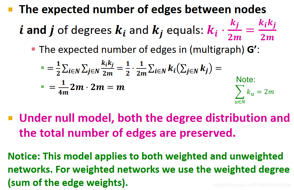
真实图共 $n$ 个节点,$m$ 条边。在 $\mathbf{G}'$ 中,节点 $i$(度数为 $k_i$)和节点 $j$(度数为 $k_j$)之间的期望边数为:$k_i\cdot\dfrac{k_j}{2m}=\dfrac{k_ik_j}{2m}$
(一共有 $2m$ 个有向边,所以一共有 $2m$ 个节点上的spoke。相当于对节点 $i$ 的 $k_i$ 个spoke每次做随机选择,每次选到 $j$ 上的spoke的概率为 $\dfrac{k_j}{2m}$)
则 $\mathbf{G}'$ 中的理想边数为:
$$\begin{aligned}
& =\frac{1}{2}\sum_{i\in N}\sum_{j\in N}\frac{k_ik_j}{2m} \\
& =\frac{1}{2}\cdot\frac{1}{2m}\sum_{i\in N}k_i(\sum_{j\in N}k_j) \\
& =\frac{1}{4m}2m\cdot 2m \\
& =m
\end{aligned}$$
所以在null model中,真实图中的度数分布和总边数都得到了保留。
(注意:这一模型可应用于有权和无权网络。对有权网络就是用有权度数(边权求和))
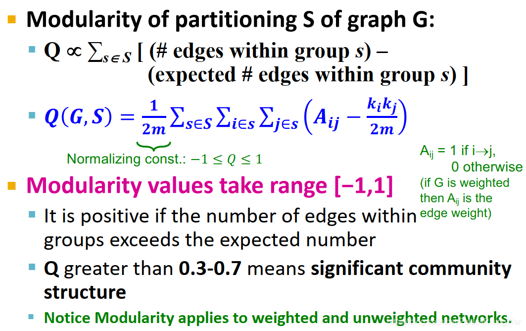
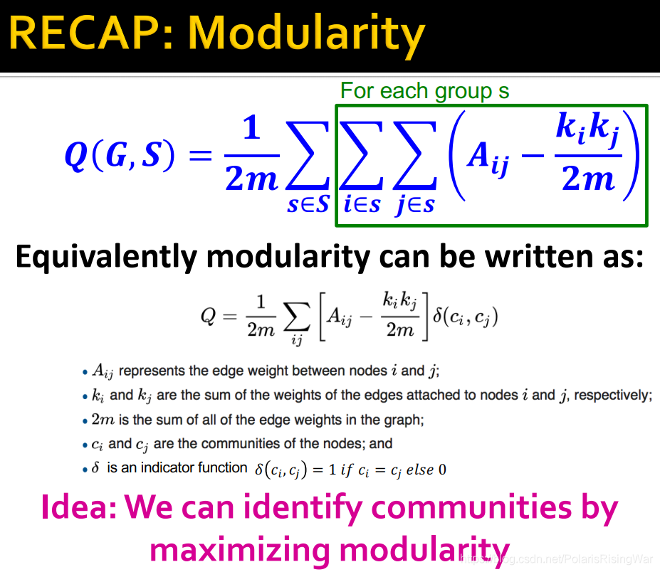
8. 所以modularity $Q(\mathbf{G},S)=\dfrac{1}{2m}\sum_{s\in S}\sum_{i\in s}\sum_{j\in s}(A_{ij}-\dfrac{k_ik_j}{2m})$
其中 $\dfrac{1}{2m}$ 是归一化常数,用于使 $-1\leq Q\leq 1$
$\begin{pmatrix}
A_{ij}= &1 &\text{if}\ i\rightarrow j, \\
&0 &\text{otherwise}
\end{pmatrix}$
(如果 $G$ 有权,$A_{ij}$ 就是边权)<br>
如果组内边数超过期望值,modularity就为正。当 $q$ 大于0.3-0.7时意味着这是个显著的社区结构。
(注意modularity概念同时可应用于有权和无权的网络)
9. modularity也可以写作:
$$Q=\frac{1}{2m}\sum_{ij}\Big[A_{ij}-\frac{k_ik_j}{2m}\Big]\delta(c_i,c_j)$$
(其中 $A_{ij}$ 是节点 $i$ 和 $j$ 之间的边权,$k_i$ 和 $k_j$ 分别是节点 $i$ 和 $j$ 入度,$2m$ 是图中边权总和,$c_i$ 和 $c_j$ 是节点所属社区,$\delta(c_i,c_j)$ 在 $c_i=c_j$ 时为1、其他时为0)
10. 我们可以通过最大化modularity来识别网络中的社区。
# 3. Louvain Algorithm
1. Louvain Algorithm
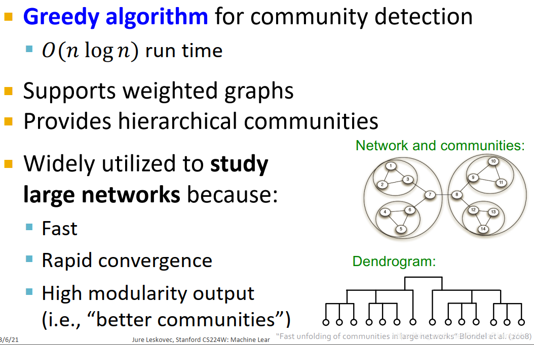
是用于社区发现的贪心算法,$O(n\log{n})$ 运行时间。
支持带权图和hierarchical社区(就可以形成如图所示的树状图dendrogram)。
广泛应用于研究大型网络,快,迅速收敛,输出的modularity高(也就意味着识别出的社区更好)。
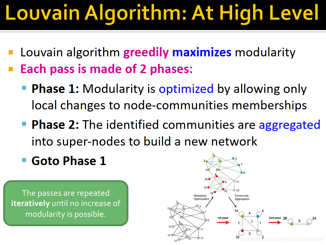
2. Louvain算法每一步分成两个阶段:
第一阶段:仅通过节点-社区隶属关系的局部改变来优化modularity。
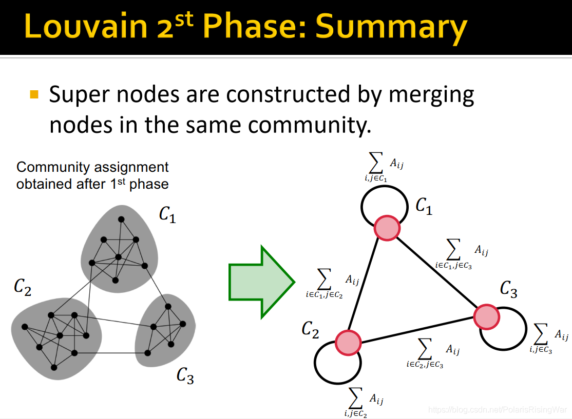
第二阶段:将第一步识别出来的communities聚合为super-nodes,从而得到一个新网络。
返回第一阶段,重复直至modularity不可能提升。
如下图右下角所示:
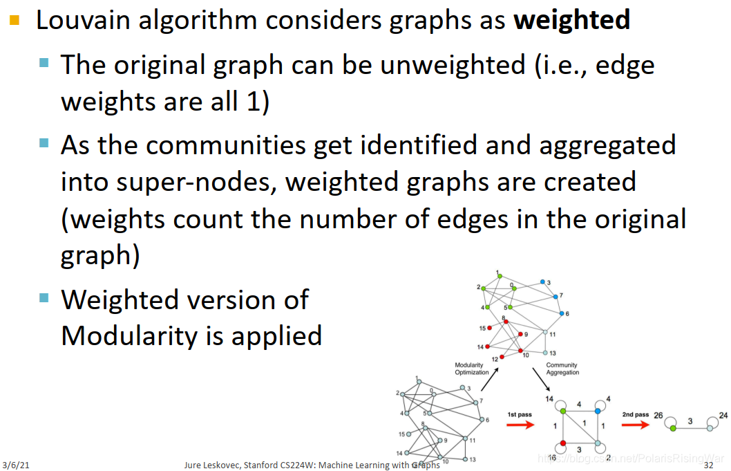
3. Louvain算法将图视作带权的。
原始图可以是无权的(例如边权全为1)。
随着社区被识别并聚合为super-nodes,算法就创造出了带权图(边权是原图中的边数)。
在计算过程中应用带权版本的modularity。
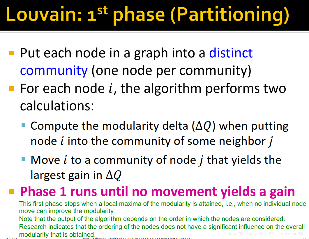
4. phase1 (partitioning)
首先将图中每个节点放到一个单独社区中(每个社区只有一个节点)。
对每个节点 $i$,计算其放到邻居 $j$ 所属节点中的 $\Delta Q$,将其放到 $\Delta Q$ 最大的 $j$ 所属的社区中。
phase1运行至调整节点社区无法得到modularity的提升(local maxima)[^9]。
注意在这个算法中,节点顺序会影响结果,但实验证明节点顺序对最终获得的总的modularity没有显著影响。
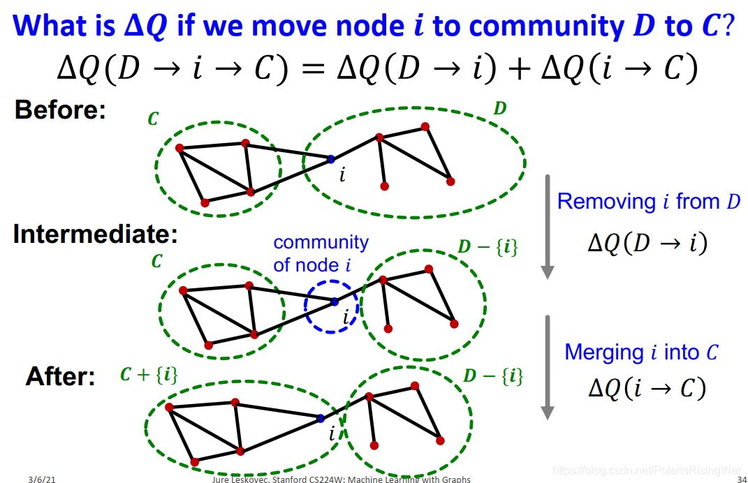
5. modularity gain
将节点 $i$ 从社区 $D$ 转移到 $C$ 的modularity gain:$\Delta Q(D\rightarrow i\rightarrow C)=\Delta Q(D\rightarrow i)+\Delta Q(i\rightarrow C)$
$\Delta Q(D\rightarrow i)$:将 $i$ 从 $D$ 中移出,单独作为一个社区
$\Delta Q(i\rightarrow C)$:将 $i$ 从单独一个社区放入 $C$ 中
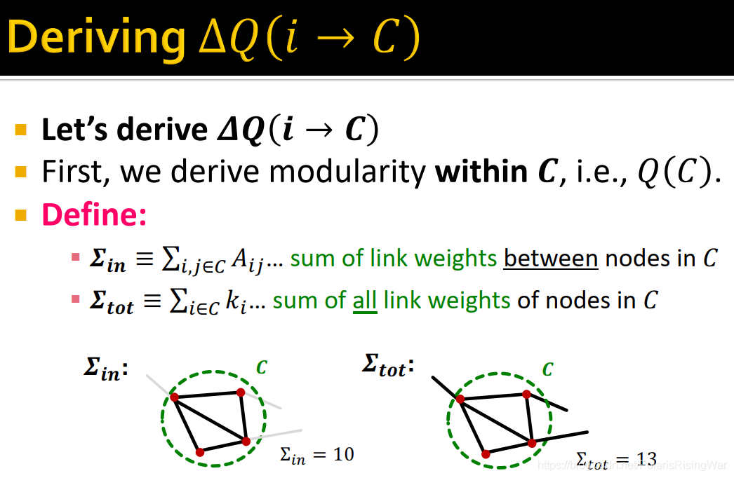
6. 接下来我们计算:$\Delta Q(i\rightarrow C)$
我们首先计算modularity winthin $C$ ($Q(C)$):
定义:
$\mathbf{\sum_{in}}\equiv\sum_{i,j\in C}A_{ij}$:$C$ 中节点间的边权总和。(如下左图,5条边,加总为10)
$\mathbf{\sum_{tot}}\equiv\sum_{i\in C}k_i$:$C$ 中节点的边权总和。
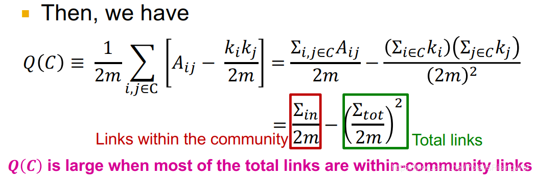
从而得到:
$$\begin{aligned}
Q(C)\equiv\frac{1}{2m}\sum_{i,j\in C}\Big[A_{ij}-\frac{k_ik_j}{2m}\Big]&=\frac{\sum_{i,j\in C}A_{ij}}{2m}-\frac{\big(\sum_{i\in C}k_i\big)\big(\sum_{j\in C} k_j\big)}{(2m)^2} \\
&=\frac{\mathbf{\sum_{in}}}{2m}-\Big(\frac{\mathbf{\sum_{tot}}}{2m}\Big)^2
\end{aligned}$$
当绝大多数链接都在社区内部时,$Q(C)$ 大。
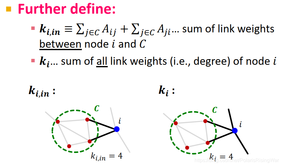
接下来我们定义:
$\mathbf{k_{i,in}}\equiv\sum_{j\in C}A_{ij}+\sum_{j\in C}A_{ji}$:节点 $i$ 和社区 $c$ 间边权加总
$\mathbf{k_i}$:节点 $i$ 边权加总(如度数)
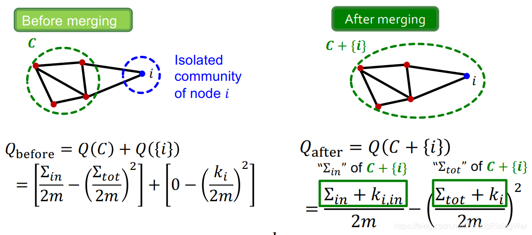
$i$ 放入 $C$ 前:
$Q_{\text{before}}=Q(C)+Q(\{i\})=\big[\frac{\mathbf{\sum_{in}}}{2m}-(\frac{\mathbf{\sum_{tot}}}{2m})^2\big]+\big[0-(\frac{k_i}{2m})^2\big]$<br>
$i$ 放入 $C$ 后:
$Q_{\text{after}}=Q(C+\{i\})=\frac{\mathbf{\sum_{in}}+k_{i,in}}{2m}-\big(\frac{\mathbf{\sum_{tot}}+k_{i}}{2m}\big)^2$
(其中 $\mathbf{\sum_{in}}+k_{i,in}$ 相当于 $\mathbf{\sum_{in}}$ of $C+\{i\}$,$\mathbf{\sum_{tot}}+k_{i}$ 相当于 $\mathbf{\sum_{tot}}$ of $C+\{i\}$)
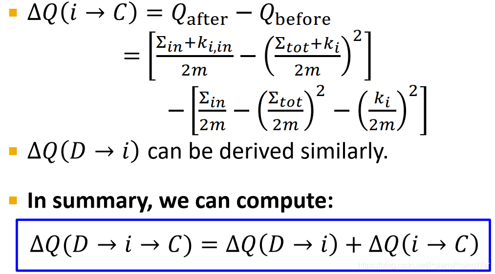
从而得到总的modularity gain:
$$\begin{aligned}
\Delta Q(i\rightarrow C)&=Q_{\text{after}}-Q_{\text{before}}\\
&=\Big[\frac{\mathbf{\sum_{in}}+k_{i,in}}{2m}-\big(\frac{\mathbf{\sum_{tot}}+k_{i}}{2m}\big)^2\Big]-\Big[\frac{\mathbf{\sum_{in}}}{2m}-(\frac{\mathbf{\sum_{tot}}}{2m})^2-(\frac{k_i}{2m})^2\Big]
\end{aligned}$$
类似地,可以得到 $\Delta Q(D\rightarrow i)$,从而得到总的 $\Delta Q(D\rightarrow i\rightarrow C)$
7. phase1总结:
迭代直至没有节点可以移动到新社区:<br>
对每个节点,计算其最优社区 $C'$:$C'=\argmax_{C'}\Delta Q(C\rightarrow i\rightarrow C')$
如果 $\Delta Q(C\rightarrow i\rightarrow C')>0$,更新社区:
$C\leftarrow C-\{i\}$
$C'\leftarrow C'+\{i\}$

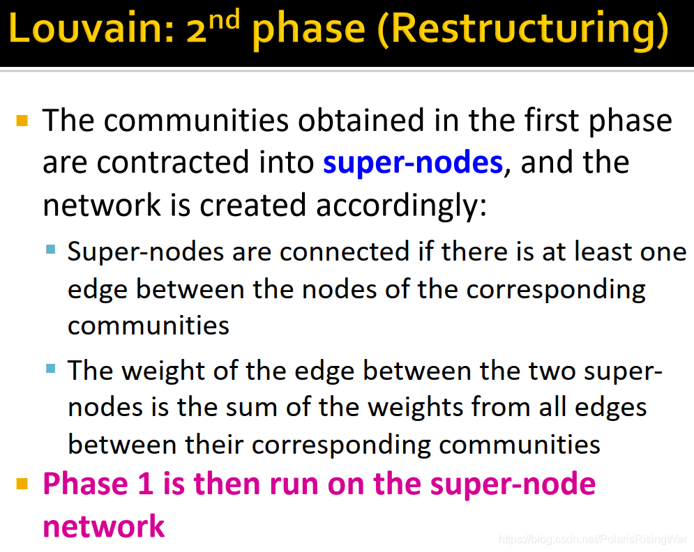
8. phase2 (restructing)
将通过上一步得到的社区收缩到super-nodes,创建新网络,如果原社区之间就有节点相连,就在对应super-nodes之间建边,边权是原对应社区之间的所有边权加总。
然后在该super-node网络上重新运行phase1
图示如下:
9. Louvain Algorithm整体图示: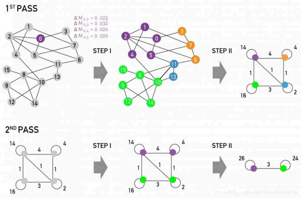
10. 在Belgian mobile phone network中,通过Louvain algorithm,可以有效划分出法语和德语社区: 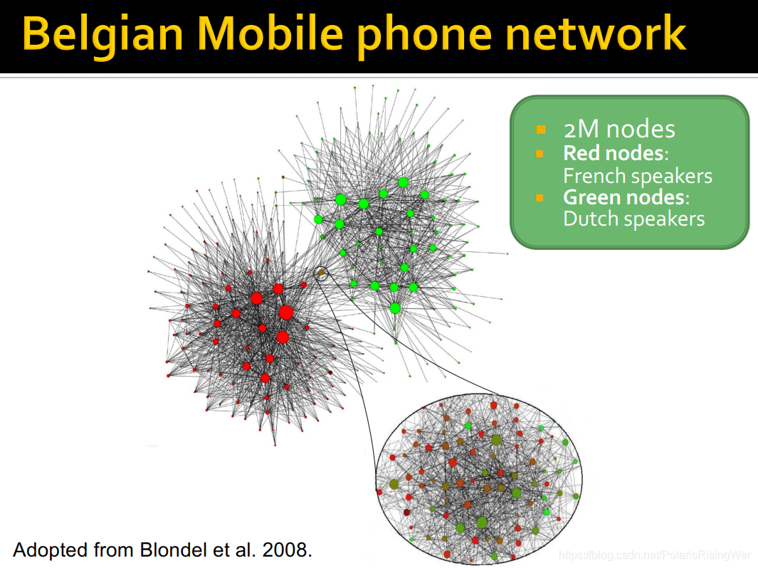
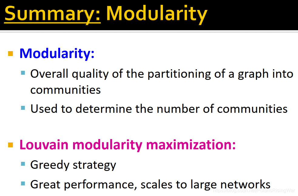
11. 本节总结
1. modularity:对将图划分到社区的partitioning的质量的评估指标,用于决定社区数
2. Louvain modularity maximization:贪心策略,表现好,能scale到大网络上
# 4. Detecting Overlapping Communities: BigCLAM
1. overlapping communities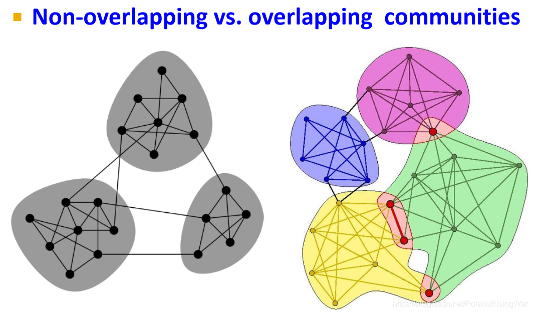
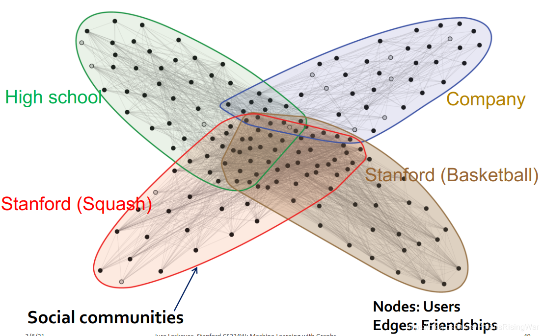
2. Facebook Ego-network[^10]
其节点是用户,边是友谊:
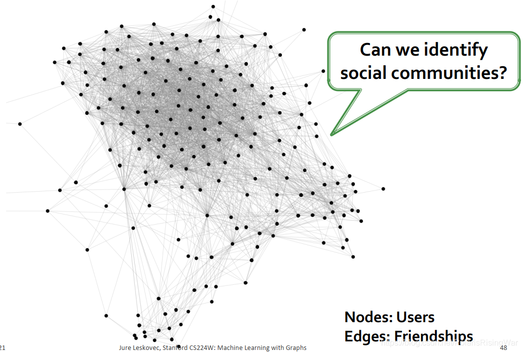
在该网络中社区之间有重叠。通过BigCLAM算法,我们可以直接通过没有任何背景知识的网络正确分类出很多节点(图中实心节点是分类正确的节点):
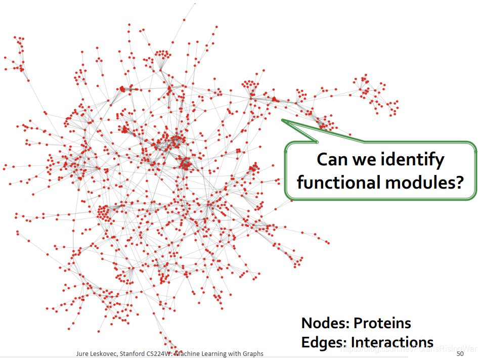
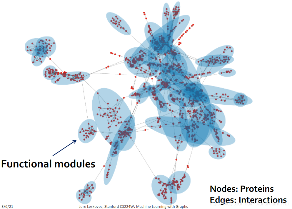
3. protein-protein interactions
在protein-protein interactions网络中,节点是蛋白质,边是interaction。其functional modules在网络中也是重叠的。
4. 重叠与非重叠的社区在图中和在邻接矩阵中的图示: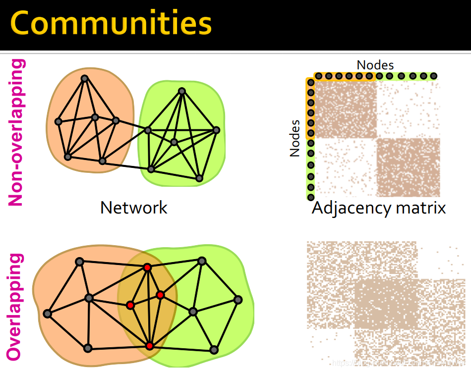
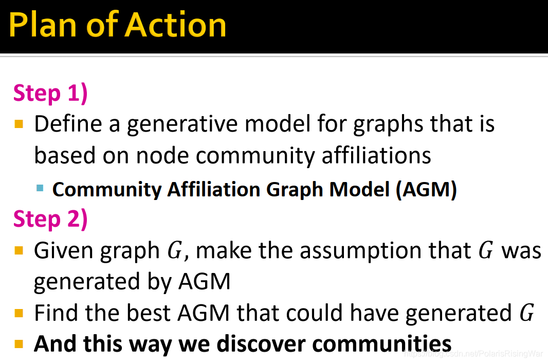
5. BigCLAM方法流程:
第一步:定义一个基于节点-社区隶属关系生成图的模型(community affiliation graph model (AGM[^12]))
第二步:给定图,假设其由AGM生成,找到最可能生成该图的AGM
通过这种方式,我们就能发现图中的社区。
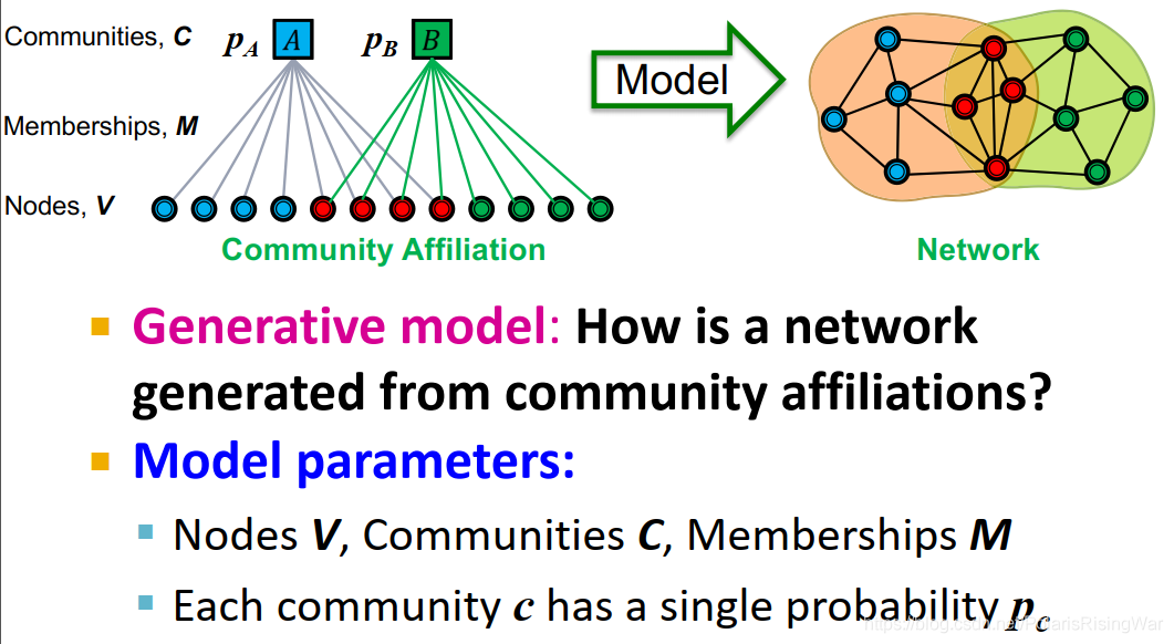
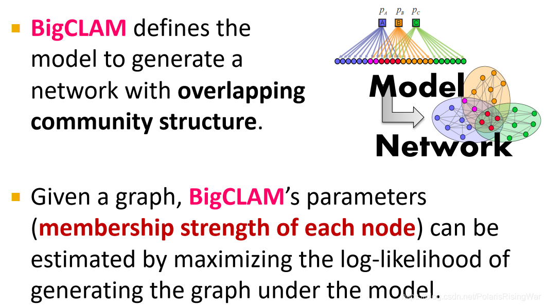
6. community affiliation graph model (AGM)
通过节点-社区隶属关系(下图左图)生成相应的网络(下图右图)。
参数为节点 $V$,社区 $C$,成员关系 $M$,每个社区 $c$ 有个概率 $p_c$
7. AGM生成图的流程
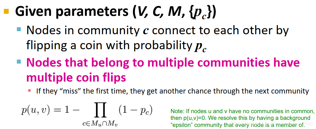
给定参数 $(V,C,M,\{p_c\})$,每个社区 $c$ 内的节点以概率 $p_c$ 互相链接。
对同属于多个社区的节点对,其相连概率就是:$p(u,v)=1-\prod\limits_{c\in M_u\cap M_v}(1-p_c)$
(注意:如果节点 $u$ 和 $v$ 没有共同社区,其相连概率就是0。为解决这一问题,我们会设置一个 background "epsilon" 社区,每个节点都属于该社区,这样每个节点都有概率相连)
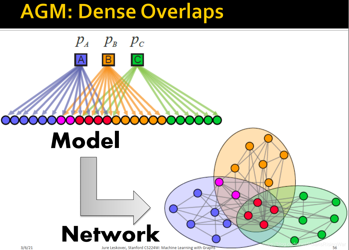
8. AGM可以生成稠密重叠的社区
9. AGM有弹性,可以生成各种社区结构:non-overlapping, overlapping, nested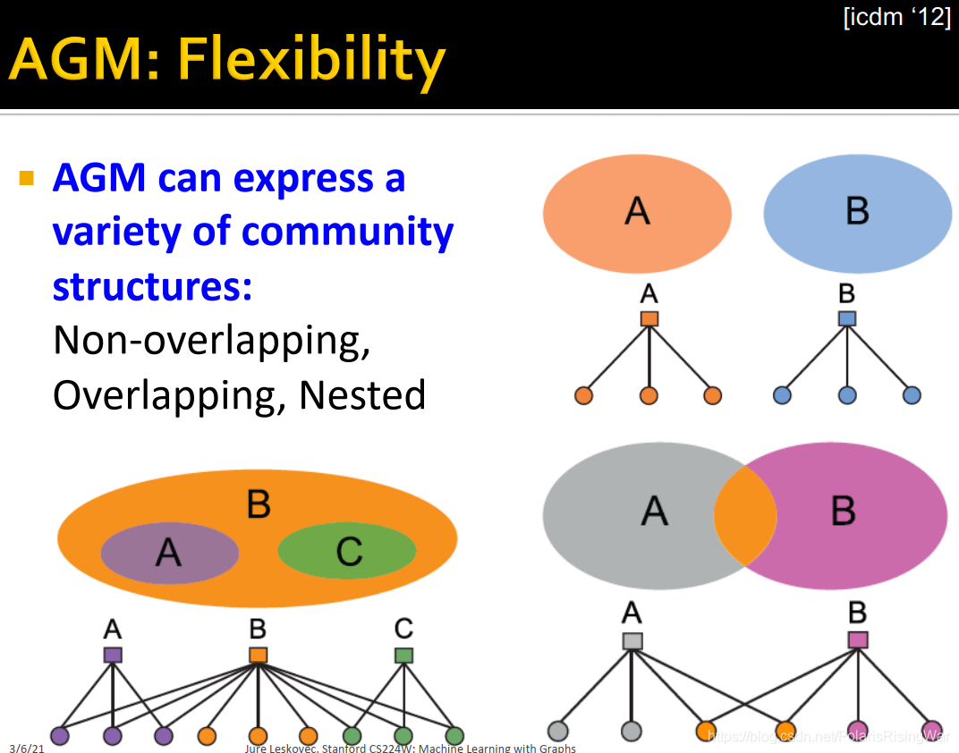
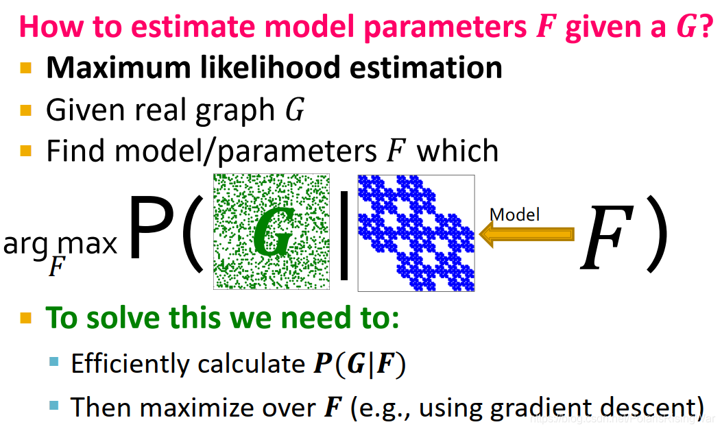
10. 通过AGM发现社区:给定图,找到最可能产生出该图的AGM模型参数(最大似然估计)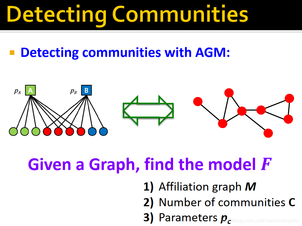
11. graph fitting
我们需要得到 $F=\argmax_FP(G|F)$
为解决这一问题,我们需要高效计算 $P(G|F)$,优化 $F$(如通过梯度下降)
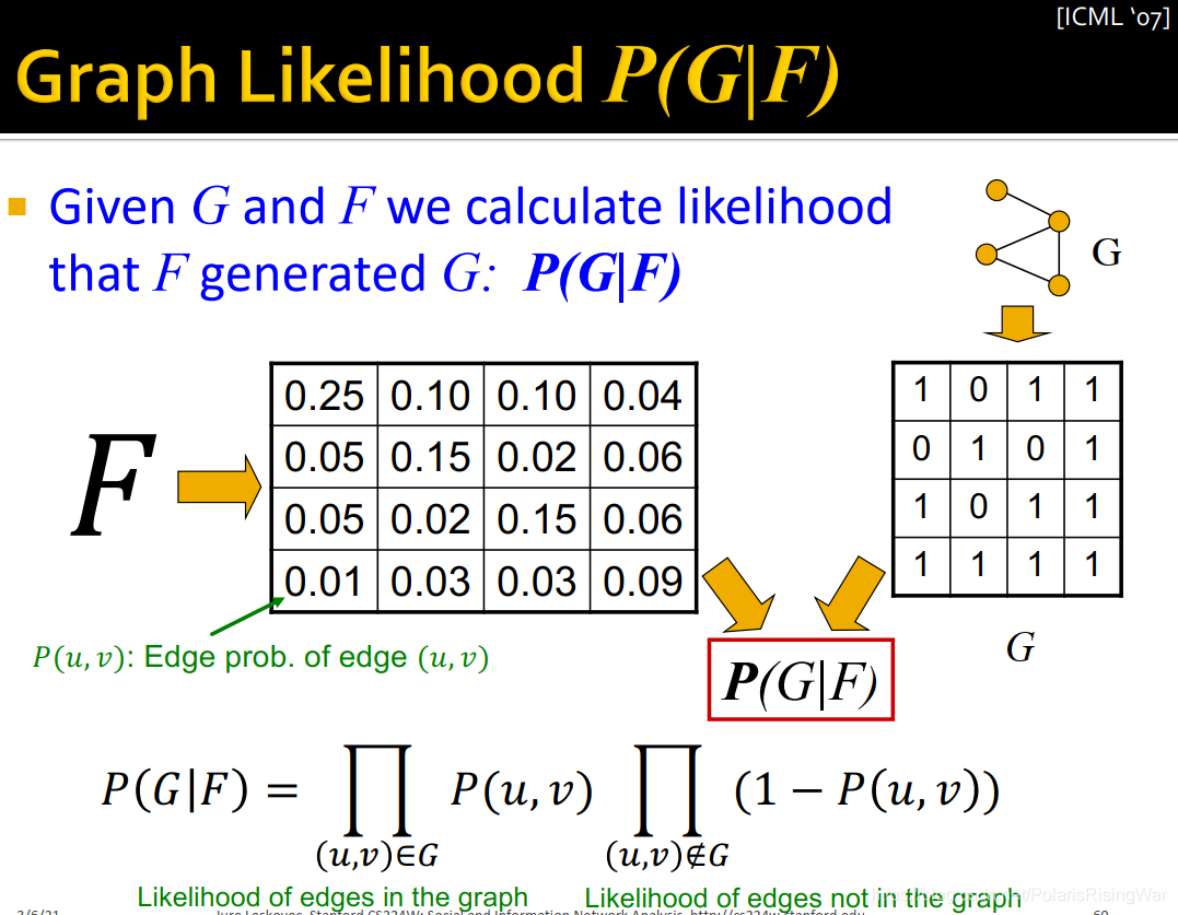
12. graph likelihood $P(G|F)$[^13]
通过 $F$ 得到边产生概率的矩阵 $P(u,v)$,$G$ 具有邻接矩阵,从而得到 $P(G|F)=\prod\limits_{(u,v)\in G}P(u,v)\prod\limits_{(u,v)\notin G}\big(1-P(u,v)\big)$
即通过AGM产生的图,原图中边存在、非边不存在的概率连乘,得到图就是原图的概率。
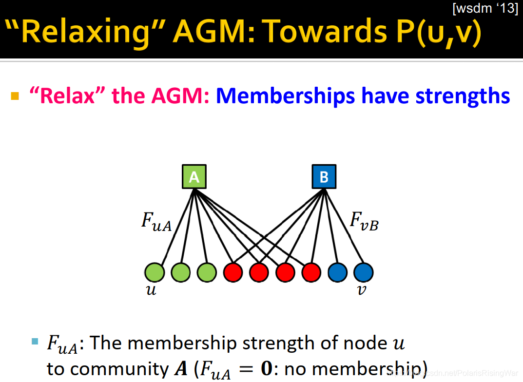
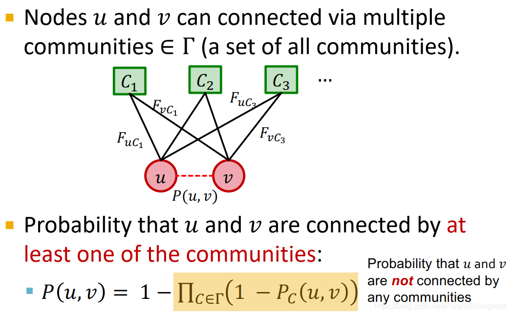
13. "Relaxing" AGM: Towards $P(u,v)$[^14]
成员关系具有strength(如图所示):$F_{uA}$ 是节点 $u$ 属于社区 $A$ 的成员关系的strength(如果 $F_{uA}=0$,说明没有成员关系)
(strength非负)
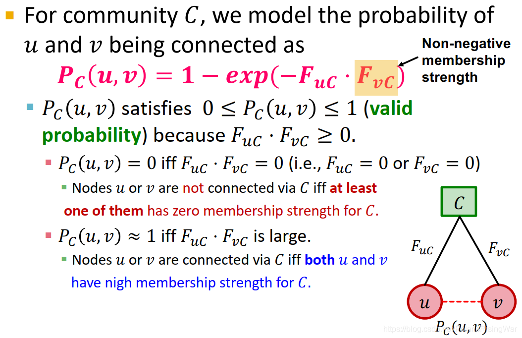
对社区 $C$,其内部节点链接概率为:$P_c(u,v)=1-\exp(-F_{uC}\cdot F_{vC})$
$0\leq P_c(u,v)\leq 1$(是个valid probability)
$P_c(u,v)=0$(节点之间无链接) 当且仅当 $F_{uC}\cdot F_{vC}=0$(至少有一个节点对 $C$ 没有成员关系)
$P_c(u,v)\approx 0$(节点之间有链接) 当且仅当 $F_{uC}\cdot F_{vC}$ 很大(两个节点都对 $C$ 有强成员关系strength)
节点对之间可以通过多个社区相连,在至少一个社区中相连,节点对就相连:
$P(u,v)=1-\prod_{C\in\Tau}\big(1-P_c(u,v)\big)$
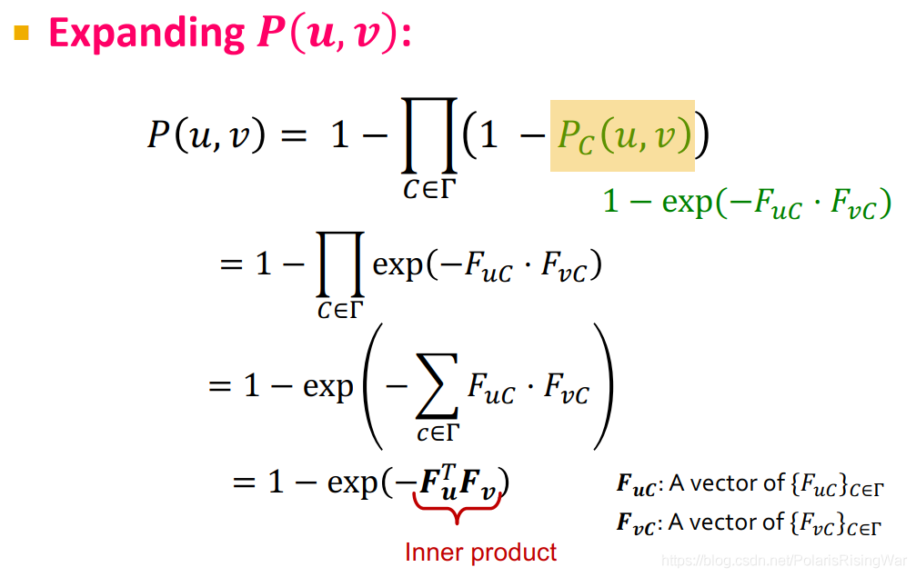
$$\begin{aligned}
P(u,v)&=1-\prod_{C\in\Tau}\big(1-P_c(u,v)\big)\\
&=1-\prod_{C\in\Tau}\Big(1-\big(1-\exp(-F_{uC}\cdot F_{vC})\big)\Big)\\
&=1-\prod_{C\in\Tau}\exp\Big(-F_{uC}\cdot F_{vC}\Big)\\
&=1-\exp\Big(-\sum\limits_{C\in\Tau}F_{uC}\cdot F_{vC}\Big)\\
&=1-\exp(-\mathbf{F}^T_u\mathbf{F}_v)\text{(内积)}
\end{aligned}$$
($\mathbf{F}_u$ 是 $\{F_{uC}\}_{C\in\Tau}$ 的向量)
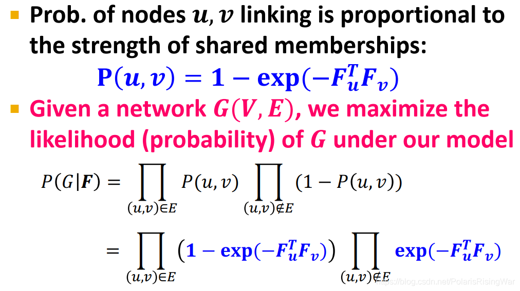
14. BigCLAM model
$\begin{aligned}
P(G|F)&=\prod\limits_{(u,v)\in E}P(u,v)\prod\limits_{(u,v)\notin E}\big(1-P(u,v)\big)\\
&=\prod\limits_{(u,v)\in E}\big(1-\exp(-\mathbf{F}^T_u\mathbf{F}_v)\big)\prod\limits_{(u,v)\notin E}\exp(-\mathbf{F}^T_u\mathbf{F}_v)
\end{aligned}$
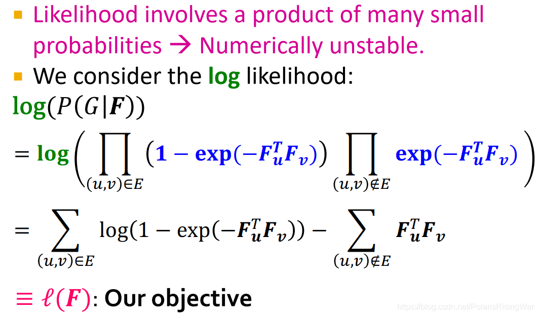
但是直接用概率的话,其值就是很多小概率相乘,数字小会导致numerically unstable的问题,所以要用log likelihood[^16](因为log是单调函数,所以可以):
$$\begin{aligned}
\log\big(P(G|F)\big)&=\log\Big(\prod\limits_{(u,v)\in E}\big(1-\exp(-\mathbf{F}^T_u\mathbf{F}_v)\big)\prod\limits_{(u,v)\notin E}\exp(-\mathbf{F}^T_u\mathbf{F}_v)\Big)\\
&=\sum_{(u,v)\in E}\log\big(1-\exp(-\mathbf{F}^T_u\mathbf{F}_v)\big)-\sum_{(u,v)\notin E}\mathbf{F}^T_u\mathbf{F}_v\\
&\equiv\mathcal{l}(F):我们的目标函数
\end{aligned}$$
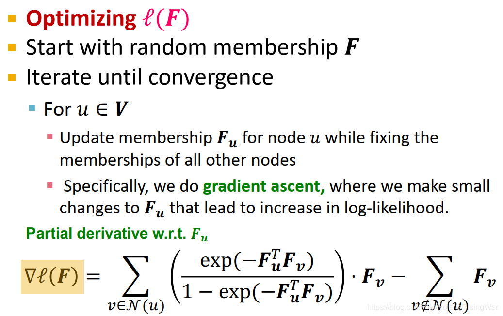
优化 $\mathcal{l}(F)$:从随机成员关系 $F$ 开始,迭代直至收敛:
对每个节点 $u$,固定其它节点的membership、更新 $F_u$。我们使用梯度提升的方法,每次对 $F_u$ 做微小修改,使log-likelihood提升。
对 $F_u$ 的偏微分[^15]:$\nabla\mathcal{l}(F)=\sum\limits_{v\in\mathcal{N}(u)}\big(\dfrac{\exp(-\mathbf{F}^T_u\mathbf{F}_v)}{1-\exp(-\mathbf{F}^T_u\mathbf{F}_v)}\big)\cdot \mathbf{F}_v-\sum\limits_{v\notin\mathcal{N}(u)}\mathbf{F}_v$
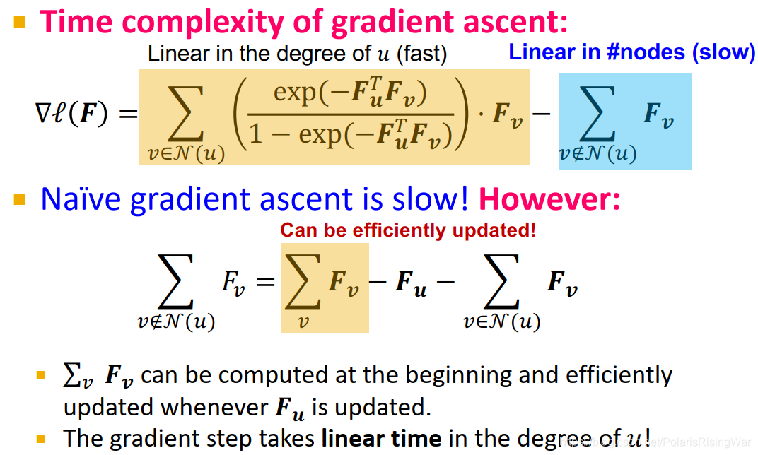
在梯度提升的过程中,$\sum\limits_{v\in\mathcal{N}(u)}\dfrac{\exp(-\mathbf{F}^T_u\mathbf{F}_v)}{1-\exp(-\mathbf{F}^T_u\mathbf{F}_v)}\cdot \mathbf{F}_v$ 与 $u$ 的度数线性相关(快),$\sum\limits_{v\notin\mathcal{N}(u)}\mathbf{F}_v$ 与图中节点数线性相关(慢)。
因此我们将后者进行分解:$\sum\limits_{v\notin\mathcal{N}(u)}\mathbf{F}_v=\sum\limits_v\mathbf{F}_v-\mathbf{F}_u-\sum\limits_{v\in\mathcal{N}(u)}\mathbf{F}_v$
右式第一项可以提前计算并cache好,每次直接用;后两项与 $u$ 的度数线性相关。
15. BigCLAM总结:
BigCLAM定义了一个模型,可生成重叠社区结构的网络。给定图,BigCLAM的参数(每个节点的membership strength)可以通过最大化对数似然估计得到。
[^1]: [Granovetter, Mark. 1973. "The Strength of Weak Ties". American Journal of Sociology 78 (May): 1360-1380](https://sociology.stanford.edu/publications/strength-weak-ties)
[^2]: 可参考我之前写的笔记:[cs224w(图机器学习)2021冬季课程学习笔记2: Traditional Methods for ML on Graphs_诸神缄默不语的博客-CSDN博客](https://blog.csdn.net/PolarisRisingWar/article/details/117336622)
[^3]: [Bearman, P.S. and Moody, J. (2004) Suicide and Friendships among American Adolescents. American Journal of Public Health, 94, 89-95.](https://www.researchgate.net/publication/8926527_Suicide_and_Friendship_Among_American_Adolescents)
[^4]: [Onnela J P , Saramki J , Hyvnen J , et al. Analysis of a large-scale weighted network of one-to-one human communication[J]. New Journal of Physics, 2007, 9(6).](http://www.cabdyn.ox.ac.uk/complexity_PDFs/Publications%202007/Onnela%20et%20al_Analysis.pdf)
[^5]: 可参考我之前写的笔记:[图数据集Zachary‘s karate club network详解,包括其在NetworkX、PyG上的获取和应用方式_诸神缄默不语的博客-CSDN博客](https://blog.csdn.net/PolarisRisingWar/article/details/117532292)
[^6]: 可参考:[模块度_百度百科](https://baike.baidu.com/item/%E6%A8%A1%E5%9D%97%E5%BA%A6)
[^7]: 可参考我之前写的笔记:[cs224w(图机器学习)2021冬季课程学习笔记15 Frequent Subgraph Mining with GNNs_诸神缄默不语的博客-CSDN博客](https://blog.csdn.net/PolarisRisingWar/article/details/119107608)
[^8]: [Meo P D , Ferrara E , Fiumara G , et al. Fast unfolding of communities in large networks. 2008.](https://arxiv.org/abs/0803.0476v2)
其他参考资料:
[Fast unfolding of communities in large networks - 知乎](https://zhuanlan.zhihu.com/p/19769897)
[Louvain 算法原理 及设计实现_xsqlx-CSDN博客_louvain算法](https://blog.csdn.net/xsqlx/article/details/79078867)
[^9]: 我有个疑惑就是,这个phase1是轮完一遍所有节点就进入phase2,还是要轮完一遍又一遍直至local maxima?反正看这里的叙述是说要轮几遍。但是我也没看过具体的代码实现,以后再看看。
[^10]: 数据集来源:[SNAP: Network datasets: Social circles](http://snap.stanford.edu/data/ego-Facebook.html)
(在本网站中有一个概念WCC,参考[^11])
ego就是用户(虽然不知道它为什么这么叫,但总之它就是这么叫),ego-network就是这个用户的社交圈(Jure在课上大概也许是这么说的这个意思)。
参考资料(没仔细看,总之列出来以资参考):
①[Chapter 9: Ego networks](http://faculty.ucr.edu/~hanneman/nettext/C9_Ego_networks.html)
②[Julian McAuley and Jure Leskovec. 2012. Learning to discover social circles in ego networks. In <i>Proceedings of the 25th International Conference on Neural Information Processing Systems - Volume 1</i> (<i>NIPS'12</i>). Curran Associates Inc., Red Hook, NY, USA, 539–547.](http://i.stanford.edu/~julian/pdfs/nips2012.pdf)
原文:

[^11]:WCC: Given a directed graph, a weakly connected component (WCC) is a subgraph of the original graph where all vertices are connected to each other by some path, ignoring the direction of edges. In case of an undirected graph, a weakly connected component is also a strongly connected component.
来源:[MADlib: Weakly Connected Components](https://madlib.apache.org/docs/latest/group__grp__wcc.html)
[^12]: [Community-Affiliation Graph Model for Overlapping Network Community Detection](https://cs.stanford.edu/~jure/pubs/agmfit-icdm12.pdf)
[^13]: 应该是这篇:[Leskovec C J . Scalable modeling of real graphs using Kronecker multiplication[C]// 2007:497--504.](https://cs.stanford.edu/~jure/pubs/kronFit-icml07.pdf)
[^14]: 应该是这篇:[Yang J , Leskovec J . Overlapping community detection at scale: A nonnegative matrix factorization approach[C]// Acm International Conference on Web Search & Data Mining. ACM, 2013.](https://cs.stanford.edu/~jure/pubs/bigclam-wsdm13.pdf)
[^15]: 这个我没自己算过,以后有缘了我来再推一遍(回忆高等数学下)
[^16]: 可参考我之前写的笔记:[cs224w(图机器学习)2021冬季课程学习笔记3: Node Embeddings](https://blog.csdn.net/PolarisRisingWar/article/details/117420662) 脚注5
