

本周早些时候,有一条推文在网上流传,其中有一段视频很好地展示了混沌动力系统的作用。
混沌的可视化:41个初始条件略有不同的三摆pic.twitter.com/CTiABFVWHW
- 费马图书馆(@fermatslibrary)2017年3月5日
编辑:有读者指出,这个动画的原创作者在2016年将其发布在reddit上。
自然,我立即想知道我是否能在Python中重现这个模拟。这个帖子就是这个结果。
这本来应该是很容易的。毕竟,不久前我写了一个Matplotlib动画教程,其中包含一个双摆的例子,在Python中使用SciPy的odeint 解算器进行模拟,并使用matplotlib的动画模块制作动画。我们需要做的就是把它扩展到一个三段摆,就可以了,对吗?
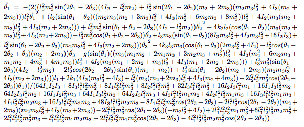
不幸的是,事情并不那么简单。虽然双摆的运动方程可以相对直接地解决,但三段摆的方程要复杂得多。例如,本文的附录中列出了支配三摆运动的三个耦合二阶微分方程;这里是这三个方程中第一个方程的截图。
幸运的是,有一些比暴力代数更简单的方法,它们依赖于更高的抽象概念:其中一种方法被称为凯恩方法。这种方法除了最微不足道的问题之外,仍然需要大量的簿记工作,但是Sympy软件包有一个很好的实现,可以为你处理这些细节。这就是我模拟三摆的方法,主要借鉴了Gede等人2013年的做法,他们提出了一个很好的应用Kane方法的Sympy的API的例子。
代码
下面的函数定义并求解了一个由任意质量和长度的n个摆组成的系统的运动方程。它有点长,但希望能有足够的注释,使你能跟上。
在[1]中
%matplotlib inline
import matplotlib.pyplot as plt
import numpy as np

from sympy import symbols
from sympy.physics import mechanics

from sympy import Dummy, lambdify
from scipy.integrate import odeint


def integrate_pendulum(n, times,
                       initial_positions=135,
                       initial_velocities=0,
                       lengths=None, masses=1):
    """Integrate a multi-pendulum with `n` sections"""
    #-------------------------------------------------
    # Step 1: construct the pendulum model

    # Generalized coordinates and velocities
    # (in this case, angular positions & velocities of each mass)
    q = mechanics.dynamicsymbols('q:{0}'.format(n))
    u = mechanics.dynamicsymbols('u:{0}'.format(n))

    # mass and length
    m = symbols('m:{0}'.format(n))
    l = symbols('l:{0}'.format(n))

    # gravity and time symbols
    g, t = symbols('g,t')

    #--------------------------------------------------
    # Step 2: build the model using Kane's Method

    # Create pivot point reference frame
    A = mechanics.ReferenceFrame('A')
    P = mechanics.Point('P')
    P.set_vel(A, 0)

    # lists to hold particles, forces, and kinetic ODEs
    # for each pendulum in the chain
    particles = []
    forces = []
    kinetic_odes = []

    for i in range(n):
        # Create a reference frame following the i^th mass
        Ai = A.orientnew('A' + str(i), 'Axis', [q[i], A.z])
        Ai.set_ang_vel(A, u[i] * A.z)

        # Create a point in this reference frame
        Pi = P.locatenew('P' + str(i), l[i] * Ai.x)
        Pi.v2pt_theory(P, A, Ai)

        # Create a new particle of mass m[i] at this point
        Pai = mechanics.Particle('Pa' + str(i), Pi, m[i])
        particles.append(Pai)

        # Set forces & compute kinematic ODE
        forces.append((Pi, m[i] * g * A.x))
        kinetic_odes.append(q[i].diff(t) - u[i])

        P = Pi

    # Generate equations of motion
    KM = mechanics.KanesMethod(A, q_ind=q, u_ind=u,
                               kd_eqs=kinetic_odes)
    fr, fr_star = KM.kanes_equations(forces, particles)

    #-----------------------------------------------------
    # Step 3: numerically evaluate equations and integrate

    # initial positions and velocities – assumed to be given in degrees
    y0 = np.deg2rad(np.concatenate([np.broadcast_to(initial_positions, n),
                                    np.broadcast_to(initial_velocities, n)]))

    # lengths and masses
    if lengths is None:
        lengths = np.ones(n) / n
    lengths = np.broadcast_to(lengths, n)
    masses = np.broadcast_to(masses, n)

    # Fixed parameters: gravitational constant, lengths, and masses
    parameters = [g] + list(l) + list(m)
    parameter_vals = [9.81] + list(lengths) + list(masses)

    # define symbols for unknown parameters
    unknowns = [Dummy() for i in q + u]
    unknown_dict = dict(zip(q + u, unknowns))
    kds = KM.kindiffdict()

    # substitute unknown symbols for qdot terms
    mm_sym = KM.mass_matrix_full.subs(kds).subs(unknown_dict)
    fo_sym = KM.forcing_full.subs(kds).subs(unknown_dict)

    # create functions for numerical calculation
    mm_func = lambdify(unknowns + parameters, mm_sym)
    fo_func = lambdify(unknowns + parameters, fo_sym)

    # function which computes the derivatives of parameters
    def gradient(y, t, args):
        vals = np.concatenate((y, args))
        sol = np.linalg.solve(mm_func(*vals), fo_func(*vals))
        return np.array(sol).T[0]

    # ODE integration
    return odeint(gradient, y0, times, args=(parameter_vals,))
提取位置
上面的函数返回广义坐标,在本例中是每个摆段的角度位置和速度,相对于垂直方向。为了使钟摆可视化,我们需要一个快速的工具来从这些角坐标中提取x和y坐标。
在[2]中
def get_xy_coords(p, lengths=None):
    """Get (x, y) coordinates from generalized coordinates p"""
    p = np.atleast_2d(p)
    n = p.shape[1] // 2
    if lengths is None:
        lengths = np.ones(n) / n
    zeros = np.zeros(p.shape[0])[:, None]
    x = np.hstack([zeros, lengths * np.sin(p[:, :n])])
    y = np.hstack([zeros, -lengths * np.cos(p[:, :n])])
    return np.cumsum(x, 1), np.cumsum(y, 1)
最后,我们可以调用这个函数来模拟一个摆在一组时间t的情况。下面是一个双摆随时间变化的路径。
在[3]中
t = np.linspace(0, 10, 1000)
p = integrate_pendulum(n=2, times=t)
x, y = get_xy_coords(p)
plt.plot(x, y);
而这里是一个三摆随时间变化的位置。
在[4]中:
p = integrate_pendulum(n=3, times=t)
x, y = get_xy_coords(p)
plt.plot(x, y);
摆锤动画
上面的静态图提供了一些情况的洞察力,但以动画的形式看结果要直观得多。借鉴我的动画教程中的双摆代码,这里有一个函数可以将摆的运动随时间的变化做成动画。
在[5]中:
from matplotlib import animation


def animate_pendulum(n):
    t = np.linspace(0, 10, 200)
    p = integrate_pendulum(n, t)
    x, y = get_xy_coords(p)

    fig, ax = plt.subplots(figsize=(6, 6))
    fig.subplots_adjust(left=0, right=1, bottom=0, top=1)
    ax.axis('off')
    ax.set(xlim=(-1, 1), ylim=(-1, 1))

    line, = ax.plot([], [], 'o-', lw=2)

    def init():
        line.set_data([], [])
        return line,

    def animate(i):
        line.set_data(x[i], y[i])
        return line,

    anim = animation.FuncAnimation(fig, animate, frames=len(t),
                                   interval=1000 * t.max() / len(t),
                                   blit=True, init_func=init)
    plt.close(fig)
    return anim
在[6]中。
anim = animate_pendulum(3)
在笔记本中,你可以用下面的片段嵌入所产生的动画。
from IPython.display import HTML
HTML(anim.to_html5_video())
像这样直接嵌入视频会导致笔记本(和博客文章!)的文件非常大,所以我已经保存了动画,并将用HTML5视频标签加载它。这样做的便携性较差(因为视频文件与笔记本是分开的),但避免了将视频的全部内容嵌入单个笔记本文件中。
In[7]:
from IPython.display import HTML
# anim.save('triple-pendulum.mp4', extra_args=['-vcodec', 'libx264'])
HTML('<video controls loop src="http://jakevdp.github.io/videos/triple-pendulum.mp4" />')
上面实现的凯恩方法的好处是,它很容易推广到更大的复合摆;例如,这里有一个5部分的 "五重摆 "的动画。它的运行时间要长一些,但可以用同样的代码计算出来。
在[8]中:
anim = animate_pendulum(5)
# HTML(anim.to_html5_video())  # uncomment to embed
在[9]中:
# anim.save('quintuple-pendulum.mp4', extra_args=['-vcodec', 'libx264'])
HTML('<video controls loop src="http://jakevdp.github.io/videos/quintuple-pendulum.mp4" />')
蝴蝶扇动它的翅膀...
现在回到这篇文章的动机:说明初始条件的小扰动的混乱结果。下面的代码将任何指定数量的几乎相同的钟摆制成动画,每个钟摆的起始位置都有轻微的扰动(这里大约是百万分之一)。
在[10]中。
from matplotlib import collections


def animate_pendulum_multiple(n, n_pendulums=41, perturbation=1E-6, track_length=15):
    oversample = 3
    track_length *= oversample

    t = np.linspace(0, 10, oversample * 200)
    p = [integrate_pendulum(n, t, initial_positions=135 + i * perturbation / n_pendulums)
         for i in range(n_pendulums)]
    positions = np.array([get_xy_coords(pi) for pi in p])
    positions = positions.transpose(0, 2, 3, 1)
    # positions is a 4D array: (npendulums, len(t), n+1, xy)

    fig, ax = plt.subplots(figsize=(6, 6))
    fig.subplots_adjust(left=0, right=1, bottom=0, top=1)
    ax.axis('off')
    ax.set(xlim=(-1, 1), ylim=(-1, 1))

    track_segments = np.zeros((n_pendulums, 0, 2))
    tracks = collections.LineCollection(track_segments, cmap='rainbow')
    tracks.set_array(np.linspace(0, 1, n_pendulums))
    ax.add_collection(tracks)

    points, = plt.plot([], [], 'ok')

    pendulum_segments = np.zeros((n_pendulums, 0, 2))
    pendulums = collections.LineCollection(pendulum_segments, colors='black')
    ax.add_collection(pendulums)

    def init():
        pendulums.set_segments(np.zeros((n_pendulums, 0, 2)))
        tracks.set_segments(np.zeros((n_pendulums, 0, 2)))
        points.set_data([], [])
        return pendulums, tracks, points

    def animate(i):
        i = i * oversample
        pendulums.set_segments(positions[:, i])
        sl = slice(max(0, i - track_length), i)
        tracks.set_segments(positions[:, sl, -1])
        x, y = positions[:, i].reshape(-1, 2).T
        points.set_data(x, y)
        return pendulums, tracks, points

    interval = 1000 * oversample * t.max() / len(t)
    anim = animation.FuncAnimation(fig, animate, frames=len(t) // oversample,
                                   interval=interval,
                                   blit=True, init_func=init)
    plt.close(fig)
    return anim

anim = animate_pendulum_multiple(3)
# HTML(anim.to_html5_video())  # uncomment to embed
在[11]中:
# anim.save('triple-pendulum-chaos.mp4', extra_args=['-vcodec', 'libx264'])
HTML('<video controls loop src="http://jakevdp.github.io/videos/triple-pendulum-chaos.mp4" />')
