本文已参与「新人创作礼」活动,一起开启掘金创作之路。
获取更多资讯,赶快关注上面的公众号吧!
【强化学习系列】
Continuous control with deep reinforcement learning
近年来,将深度学习与强化学习相结合的方法取得了显著的进展,“深度Q网络”(Deep Q Network, DQN)算法能够在许多雅达利(Atari)视频游戏中使用未经处理的像素作为输入,就达到人类水平的性能,其中使用深度神经网络函数逼近器来估计动作值函数。
然而,DQN在解决高维观察空间问题的同时,只能处理离散的、低维的动作空间。许多有趣的任务,尤其是物理控制任务,都具有连续的(实值)和高维的动作空间。DQN不能直接应用于连续域,因为它依赖于找到最大化动作值函数的动作,而在连续值情况下,为找到这个动作,每一步都需要进行迭代优化。
将深度强化学习方法(如DQN)应用于连续域的一种显而易见的方法就是是对动作空间进行简单的离散化。然而,该方法也有许多限制,最明显的是维数灾难:动作的数量随着自由度的增加呈指数增长。例如,对于一个7自由度的机械臂,对其进行粗糙的离散化,假设每个关节仅有ai∈{−k,0,k}三个可选动作,那么整个系统的动作空间维度为:3^7^=2187。如此大的动作空间很难有效地探索,因此在这种情况下成功地训练类似DQN的网络可能很困难。此外,这种主观的离散化势必会丢弃部分动作域的结构信息,而这些信息对求解很多问题都很重要,也就是说这种人为的离散化可能导致求解精度的降低。
所以是不是有更好的解决连续动作空间问题的方法呢?
今天就介绍一种使用深度强化学习进行连续控制的文章——《Continuous control with deep reinforcement learning》,这篇文章是由Google Deepmind于2015年发表的,文中提出了一种基于确定性策略梯度的演员-评论家无模型离策略算法,使用深度函数逼近学习高维、连续动作空间下的策略。演员-评论家可以用于解决连续动作空间问题,DQN则通过经验回放和目标网络实现稳定、鲁棒的学习值函数,该算法结合了演员-评论家方法和DQN,集众家之所长,可以在连续动作空间问题上具有很好的表现,实验结果也表明该算法可以非常鲁棒地解决20多种模拟物理任务。
下面将介绍一下该算法的原理和代码实现。
1.1 基础
通常环境是部分可观的,所以需要整个历史的观察-动作对st=(x1,a1,…,at−1,xt)来描述状态,这里假设环境满足马尔科夫属性st=xt。
策略Π为将状态映射为动作的概率分布:π:S→P(A)。
从某一状态的回报为折扣未来奖励总和Rt=∑i=tTγ(i−t)r(si,ai)。注意,回报取决于所选择的动作,也就依赖于策略,因此可能也是随机的,强化学习的目标是学习一个策略以最大化从起始状态开始获取的期望回报Eπ[R1]。
在许多强化学习算法中都是用动作值函数,它描述了从状态St开始采取at之后遵循策略π所能获得的期望回报:
Q^{\pi}\left(s_{t}, a_{t}\right)=\mathbb{E}_{r_{i \geq t}, s_{i>t} \sim E, a_{i>t} \sim \pi}\left[R_{t} | s_{t}, a_{t}\right]\tag{1}
强化学习中的许多方法都是使用了贝尔曼等式进行迭代:
Q^{\pi}\left(s_{t}, a_{t}\right)=\mathbb{E}_{r_{t}, s_{t+1} \sim E}\left[r\left(s_{t}, a_{t}\right)+\gamma \mathbb{E}_{a_{t+1} \sim \pi}\left[Q^{\pi}\left(s_{t+1}, a_{t+1}\right)\right]\right]\tag{2}
如果目标策略是确定性的,可以将其描述为一个函数μ:S←A,从而将内部的期望移掉:
Q^{\mu}\left(s_{t}, a_{t}\right)=\mathbb{E}_{r_{t}, s_{t+1} \sim E}\left[r\left(s_{t}, a_{t}\right)+\gamma Q^{\mu}\left(s_{t+1}, \mu\left(s_{t+1}\right)\right)\right]\tag{3}
注意到外层的期望仅仅依赖环境,这意味着可以通过来自另一个不同的策略的β的转移来学习离策略Qμ。考虑参数为θQ的函数逼近,通过最小化损失进行优化:
L\left(\theta^{Q}\right)=\mathbb{E}_{s_{t} \sim \rho^{\beta}, a_{t} \sim \beta, r_{t} \sim E}\left[\left(Q\left(s_{t}, a_{t} | \theta^{Q}\right)-y_{t}\right)^{2}\right]\tag{4}s
其中
y_{t}=r\left(s_{t}, a_{t}\right)+\gamma Q\left(s_{t+1}, \mu\left(s_{t+1}\right) | \theta^{Q}\right)\tag{5}
1.2 算法
前面已经提到,无法直接应用Q学习解决连续动作空间问题,因为在连续空间内寻找贪婪策略需要每一时间步进行at的优化,对于大规模、无约束的函数逼近器和重要的动作空间,这种优化太过缓慢而不实用,相反,这里使用了基于DPG的演员-评论家算法。
确定性策略梯度DPG使用了一个参数化的演员函数μ(s∣θμ),该函数可以确定性地将状态映射为某一特定的动作。评论家Q(s,a)使用如Q学习中的贝尔曼等式进行学习。演员通过在等式(3)上应用链式规则更新其参数:
\nabla_{\theta^{\mu}} J & \approx \mathbb{E}_{\boldsymbol{s}_{\boldsymbol{t}} \sim \boldsymbol{\rho}^{\beta}}\left[\left.\nabla_{\theta^{\mu}} Q\left(s, a | \theta^{Q}\right)\right|_{s=s_{t}, a=\mu\left(s_{t} | \theta^{\mu}\right)}\right] \\
&=\mathbb{E}_{\boldsymbol{s}_{\boldsymbol{t}} \sim \boldsymbol{\rho}^{\beta}}\left[\left.\left.\nabla_{a} Q\left(s, a | \theta^{Q}\right)\right|_{s=s_{t}, a=\mu\left(s_{t}\right)} \nabla_{\theta_{\mu}} \mu\left(s | \theta^{\mu}\right)\right|_{s=s_{t}}\right]
\end{aligned}\tag{6}$$
  Silver已经证明这就是策略梯度,也就是策略在整体性能上的梯度(详见 [第十三章 确定性策略梯度(Deterministic Policy Gradient Algorithms,DPG)-强化学习理论学习与代码实现(强化学习导论第二版)](https://blog.csdn.net/hba646333407/article/details/105584029))。<br>
  本文作者的贡献是受DQN的启发对DPG进行了改进,允许使用神经网络函数逼近器有效地在大状态和动作空间进行在线学习,并将这种算法称为深度确定性策略Deep DPG(DDPG)。<br>
  将神经网络用于强化学习可能存在的问题是,大多数优化算法都假设了样本是独立同分布的,但是很显然,当在环境中按顺序探索生成样本时,这个假设不再成立,因为样本前后存在相关性,此外为了充分利用硬件优化,以最小批进行学习比在线学习更重要。<br>
  同DQN一样,这里也引入了经验回放来解决这个问题,经验回放就是一个有限大小的缓存$\mathcal{R}$。根据探索策略从环境中采样变迁,然后把元组$\left(s_{t}, a_{t}, r_{t}, s_{t+1}\right)$存入经验回放中,在每一时间步,演员和评论家通过从中随机均匀采样一小批量进行更新。<br>
  直接实现神经网络逼近的Q学习(等式4)被证明在很多环境下是不稳定的。由于被更新的网络$Q\left(s, a | \theta^{Q}\right)$同样会用于计算目标Q值(等式5),所以Q值更新很容易发散。解决方法就是引入目标网络,但是针对演员-批评家进行了修改,并使用“软”目标更新,并不是直接复制权重。分别为演员和评论家网络创建了一个副本$Q^{\prime}\left(s, a | \theta^{Q^{\prime}}\right)$和$\mu^{\prime}\left(s | \theta^{\mu^{\prime}}\right)$,用于计算目标值,然后通过让这些目标网络缓慢地跟踪学习网络来更新它们的权重:$\theta^{\prime} \leftarrow \tau \theta+(1-\tau) \theta^{\prime}$ with $\tau \ll 1$,从而限制目标值缓慢变化,这大大提高了学习的稳定性,所以在DDPG中一共有4个网络。<br>
  在连续行动空间中学习的一个主要挑战是有效地探索。像DDPG这样的off-policy算法的一个优点是,可以独立于学习算法来处理探索问题。通过在演员策略上添加噪声$\mathcal{N}$来构造探索策略$\mu^{\prime}$:
$$\mu^{\prime}\left(s_{t}\right)=\mu\left(s_{t} | \theta_{t}^{\mu}\right)+\mathcal{N}\tag{7}$$
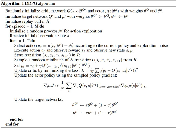
<center>图1 DDPG算法</center>
## 1.3 算法和网络结构分析
  DDPG吸收了演员-评论家(Actor-Critic)让策略梯度单步更新的优点,而且还吸收了让计算机学会玩游戏的DQN的,我们将DDPG分成‘Deep’和‘Deterministic Policy Gradient’,然后‘Deterministic Policy Gradient’又能被细分为‘Deterministic’和‘Policy Gradient’,通过这样的分解分析,就可以很快搞清楚DDPG的原理了。<br>
  深度Deep:顾名思义,使用更深层次的神经网络作为函数逼近器,在DQN中使用经验回放和两套结构相同,但参数更新频率不同的神经网络能有效促进学习。那我们也把这种思想运用到DDPG 当中,使DDPG 也具备这种优良形式。<br>
  Policy gradient:相比其他的强化学习方法,策略梯度能被用来在连续动作上进行动作的筛选,而且筛选的时候是根据所学习到的动作分布随机进行筛选,也就是说最终给出的是每个动作的概率,通过该概率选择动作。<br>
  Deterministic:由于Policy gradient输出的是一个不确定的概率分布,那确定性就是说在做动作的时候没必要那么不确定,反正最终都只是要输出一个动作值,不必随机,不如直接铁定一点。所以Deterministic就改变了输出动作的过程,直截了当地只在连续动作上输出一个动作值。<br>
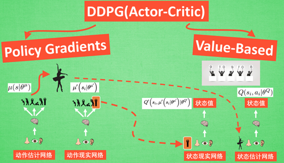
<center>图2 DDPG网络结构(图片更改自莫烦PYTHON)</center>
  现在我们来说说DDPG中所用到的神经网络。它其实和我们之前提到的Actor-Critic形式差不多,也需要有基于策略Policy的神经网络和基于价值Value的神经网络,但是为了体现DQN的思想,也就是为了使更新目标更加稳定,每种神经网络我们都需要再细分为两个,Policy Gradient这边,有估计网络和现实网络,估计网络用来输出实时的动作,供actor在现实中实行;而现实网络则是用来更新价值网络系统的。所以我们再来看看价值系统这边,同样也有现实网络和估计网络,他们都在输出这个状态的价值,而输入端却有不同,状态现实网络这边会拿着从动作现实网络来的动作加上状态的观测值加以分析,而状态估计网络则是拿着当时Actor施加的动作当做输入。在实际运用中,DDPG的这种做法的确带来了更有效的学习过程。
## 1.4 代码实现
```python
"""
Deep Deterministic Policy Gradient (DDPG), Reinforcement Learning.
DDPG is Actor Critic based algorithm.
Pendulum example.
View more on my tutorial page: https://morvanzhou.github.io/tutorials/
Using:
tensorflow 1.0
gym 0.8.0
"""
import tensorflow as tf
import numpy as np
import gym
import time
np.random.seed(1)
tf.set_random_seed(1)
##################### hyper parameters ####################
MAX_EPISODES = 200
MAX_EP_STEPS = 200
LR_A = 0.001 # learning rate for actor
LR_C = 0.001 # learning rate for critic
GAMMA = 0.9 # reward discount
REPLACEMENT = [
dict(name='soft', tau=0.01),
dict(name='hard', rep_iter_a=600, rep_iter_c=500)
][0] # you can try different target replacement strategies
MEMORY_CAPACITY = 10000
BATCH_SIZE = 32
RENDER = False
OUTPUT_GRAPH = True
ENV_NAME = 'Pendulum-v0'
############################### Actor ####################################
class Actor(object):
def __init__(self, sess, action_dim, action_bound, learning_rate, replacement):
self.sess = sess
self.a_dim = action_dim
self.action_bound = action_bound
self.lr = learning_rate
self.replacement = replacement
self.t_replace_counter = 0
with tf.variable_scope('Actor'):
# input s, output a
self.a = self._build_net(S, scope='eval_net', trainable=True)
# input s_, output a, get a_ for critic
self.a_ = self._build_net(S_, scope='target_net', trainable=False)
self.e_params = tf.get_collection(tf.GraphKeys.GLOBAL_VARIABLES, scope='Actor/eval_net')
self.t_params = tf.get_collection(tf.GraphKeys.GLOBAL_VARIABLES, scope='Actor/target_net')
if self.replacement['name'] == 'hard':
self.t_replace_counter = 0
self.hard_replace = [tf.assign(t, e) for t, e in zip(self.t_params, self.e_params)]
else:
self.soft_replace = [tf.assign(t, (1 - self.replacement['tau']) * t + self.replacement['tau'] * e)
for t, e in zip(self.t_params, self.e_params)]
def _build_net(self, s, scope, trainable):
with tf.variable_scope(scope):
init_w = tf.random_normal_initializer(0., 0.3)
init_b = tf.constant_initializer(0.1)
net = tf.layers.dense(s, 30, activation=tf.nn.relu,
kernel_initializer=init_w, bias_initializer=init_b, name='l1',
trainable=trainable)
with tf.variable_scope('a'):
actions = tf.layers.dense(net, self.a_dim, activation=tf.nn.tanh, kernel_initializer=init_w,
bias_initializer=init_b, name='a', trainable=trainable)
scaled_a = tf.multiply(actions, self.action_bound, name='scaled_a') # Scale output to -action_bound to action_bound
return scaled_a
def learn(self, s): # batch update
self.sess.run(self.train_op, feed_dict={S: s})
if self.replacement['name'] == 'soft':
self.sess.run(self.soft_replace)
else:
if self.t_replace_counter % self.replacement['rep_iter_a'] == 0:
self.sess.run(self.hard_replace)
self.t_replace_counter += 1
def choose_action(self, s):
s = s[np.newaxis, :] # single state
return self.sess.run(self.a, feed_dict={S: s})[0] # single action
def add_grad_to_graph(self, a_grads):
with tf.variable_scope('policy_grads'):
# ys = policy;
# xs = policy's parameters;
# a_grads = the gradients of the policy to get more Q
# tf.gradients will calculate dys/dxs with a initial gradients for ys, so this is dq/da * da/dparams
self.policy_grads = tf.gradients(ys=self.a, xs=self.e_params, grad_ys=a_grads)
with tf.variable_scope('A_train'):
opt = tf.train.AdamOptimizer(-self.lr) # (- learning rate) for ascent policy
self.train_op = opt.apply_gradients(zip(self.policy_grads, self.e_params))
############################### Critic ####################################
class Critic(object):
def __init__(self, sess, state_dim, action_dim, learning_rate, gamma, replacement, a, a_):
self.sess = sess
self.s_dim = state_dim
self.a_dim = action_dim
self.lr = learning_rate
self.gamma = gamma
self.replacement = replacement
with tf.variable_scope('Critic'):
# Input (s, a), output q
self.a = tf.stop_gradient(a) # stop critic update flows to actor
self.q = self._build_net(S, self.a, 'eval_net', trainable=True)
# Input (s_, a_), output q_ for q_target
self.q_ = self._build_net(S_, a_, 'target_net', trainable=False) # target_q is based on a_ from Actor's target_net
self.e_params = tf.get_collection(tf.GraphKeys.GLOBAL_VARIABLES, scope='Critic/eval_net')
self.t_params = tf.get_collection(tf.GraphKeys.GLOBAL_VARIABLES, scope='Critic/target_net')
with tf.variable_scope('target_q'):
self.target_q = R + self.gamma * self.q_
with tf.variable_scope('TD_error'):
self.loss = tf.reduce_mean(tf.squared_difference(self.target_q, self.q))
with tf.variable_scope('C_train'):
self.train_op = tf.train.AdamOptimizer(self.lr).minimize(self.loss)
with tf.variable_scope('a_grad'):
self.a_grads = tf.gradients(self.q, self.a)[0] # tensor of gradients of each sample (None, a_dim)
if self.replacement['name'] == 'hard':
self.t_replace_counter = 0
self.hard_replacement = [tf.assign(t, e) for t, e in zip(self.t_params, self.e_params)]
else:
self.soft_replacement = [tf.assign(t, (1 - self.replacement['tau']) * t + self.replacement['tau'] * e)
for t, e in zip(self.t_params, self.e_params)]
def _build_net(self, s, a, scope, trainable):
with tf.variable_scope(scope):
init_w = tf.random_normal_initializer(0., 0.1)
init_b = tf.constant_initializer(0.1)
with tf.variable_scope('l1'):
n_l1 = 30
w1_s = tf.get_variable('w1_s', [self.s_dim, n_l1], initializer=init_w, trainable=trainable)
w1_a = tf.get_variable('w1_a', [self.a_dim, n_l1], initializer=init_w, trainable=trainable)
b1 = tf.get_variable('b1', [1, n_l1], initializer=init_b, trainable=trainable)
net = tf.nn.relu(tf.matmul(s, w1_s) + tf.matmul(a, w1_a) + b1)
with tf.variable_scope('q'):
q = tf.layers.dense(net, 1, kernel_initializer=init_w, bias_initializer=init_b, trainable=trainable) # Q(s,a)
return q
def learn(self, s, a, r, s_):
self.sess.run(self.train_op, feed_dict={S: s, self.a: a, R: r, S_: s_})
if self.replacement['name'] == 'soft':
self.sess.run(self.soft_replacement)
else:
if self.t_replace_counter % self.replacement['rep_iter_c'] == 0:
self.sess.run(self.hard_replacement)
self.t_replace_counter += 1
##################### Memory ####################
class Memory(object):
def __init__(self, capacity, dims):
self.capacity = capacity
self.data = np.zeros((capacity, dims))
self.pointer = 0
def store_transition(self, s, a, r, s_):
transition = np.hstack((s, a, [r], s_))
index = self.pointer % self.capacity # replace the old memory with new memory
self.data[index, :] = transition
self.pointer += 1
def sample(self, n):
assert self.pointer >= self.capacity, 'Memory has not been fulfilled'
indices = np.random.choice(self.capacity, size=n)
return self.data[indices, :]
env = gym.make(ENV_NAME)
env = env.unwrapped
env.seed(1)
state_dim = env.observation_space.shape[0]
action_dim = env.action_space.shape[0]
action_bound = env.action_space.high
# all placeholder for tf
with tf.name_scope('S'):
S = tf.placeholder(tf.float32, shape=[None, state_dim], name='s')
with tf.name_scope('R'):
R = tf.placeholder(tf.float32, [None, 1], name='r')
with tf.name_scope('S_'):
S_ = tf.placeholder(tf.float32, shape=[None, state_dim], name='s_')
sess = tf.Session()
# Create actor and critic.
# They are actually connected to each other, details can be seen in tensorboard or in this picture:
actor = Actor(sess, action_dim, action_bound, LR_A, REPLACEMENT)
critic = Critic(sess, state_dim, action_dim, LR_C, GAMMA, REPLACEMENT, actor.a, actor.a_)
actor.add_grad_to_graph(critic.a_grads)
sess.run(tf.global_variables_initializer())
M = Memory(MEMORY_CAPACITY, dims=2 * state_dim + action_dim + 1)
if OUTPUT_GRAPH:
tf.summary.FileWriter("logs/", sess.graph)
var = 3 # control exploration
t1 = time.time()
for i in range(MAX_EPISODES):
s = env.reset()
ep_reward = 0
for j in range(MAX_EP_STEPS):
if RENDER:
env.render()
# Add exploration noise
a = actor.choose_action(s)
a = np.clip(np.random.normal(a, var), -2, 2) # add randomness to action selection for exploration
s_, r, done, info = env.step(a)
M.store_transition(s, a, r / 10, s_)
if M.pointer > MEMORY_CAPACITY:
var *= .9995 # decay the action randomness
b_M = M.sample(BATCH_SIZE)
b_s = b_M[:, :state_dim]
b_a = b_M[:, state_dim: state_dim + action_dim]
b_r = b_M[:, -state_dim - 1: -state_dim]
b_s_ = b_M[:, -state_dim:]
critic.learn(b_s, b_a, b_r, b_s_)
actor.learn(b_s)
s = s_
ep_reward += r
if j == MAX_EP_STEPS-1:
print('Episode:', i, ' Reward: %i' % int(ep_reward), 'Explore: %.2f' % var, )
if ep_reward > -300:
RENDER = True
break
print('Running time: ', time.time()-t1)
```


