

当我们从事与图像有关的机器学习问题时,不仅需要收集一些图像作为训练数据,还需要采用增强的方式来创造图像的变化。这对于比较复杂的物体识别问题来说尤其如此。
有很多方法可以进行图像增强。你可以使用一些外部库或者自己编写函数来实现。在TensorFlow和Keras中也有一些用于增强的模块。在这篇文章中,你会发现我们如何使用Keras的预处理层以及TensorFlow中的tf.image 模块来进行图像增强。
读完这篇文章,你会知道:
- 什么是Keras的预处理层以及如何使用它们
tf.image模块为图像增强提供的功能是什么?- 如何将增强功能与
tf.data数据集一起使用。
让我们开始吧。
概述
本文分为五个部分,它们是:
- 获取图像
- 图像的可视化
- Keras预处理Layesr
- 使用tf.image API进行扩增
- 在神经网络中使用预处理层
获取图像
在我们看到如何进行增强之前,我们需要获得图像。最终,我们需要将图像表示为数组,例如,以HxWx3的8位整数表示RGB像素值。有许多方法可以获得图像。有些可以以ZIP文件的形式下载。如果你使用TensorFlow,你可以从tensorflow_datasets 库中获得一些图像数据集。
在本教程中,我们将使用柑橘叶子的图像,这是一个小于100MB的小数据集。它可以从tensorflow_datasets ,如下所示。
import tensorflow_datasets as tfds
ds, meta = tfds.load('citrus_leaves', with_info=True, split='train', shuffle_files=True)
第一次运行这段代码将把图像数据集下载到你的计算机中,输出结果如下。
Downloading and preparing dataset 63.87 MiB (download: 63.87 MiB, generated: 37.89 MiB, total: 101.76 MiB) to ~/tensorflow_datasets/citrus_leaves/0.1.2...
Extraction completed...: 100%|██████████████████████████████| 1/1 [00:06<00:00,  6.54s/ file]
Dl Size...: 100%|██████████████████████████████████████████| 63/63 [00:06<00:00,  9.63 MiB/s]
Dl Completed...: 100%|███████████████████████████████████████| 1/1 [00:06<00:00,  6.54s/ url]
Dataset citrus_leaves downloaded and prepared to ~/tensorflow_datasets/citrus_leaves/0.1.2. Subsequent calls will reuse this data.
上面的函数将图像作为一个tf.data 数据集对象和元数据返回。这是一个分类数据集。我们可以用下面的方法打印训练标签。
...
for i in range(meta.features['label'].num_classes):
    print(meta.features['label'].int2str(i))
并且这样打印。
Black spot
canker
greening
healthy
如果你以后再运行这段代码,你将重新使用下载的图像。但另一种将下载的图像加载到tf.data 数据集的方法是image_dataset_from_directory() 函数。
我们可以看到上面的屏幕输出,数据集被下载到目录~/tensorflow_datasets 。如果你看一下这个目录,你会看到目录结构如下。
.../Citrus/Leaves
├── Black spot
├── Melanose
├── canker
├── greening
└── healthy
这些目录是标签,图像是存储在其相应目录下的文件。我们可以让函数将目录递归地读入数据集。
import tensorflow as tf
from tensorflow.keras.utils import image_dataset_from_directory

# set to fixed image size 256x256
PATH = ".../Citrus/Leaves"
ds = image_dataset_from_directory(PATH,
                                  validation_split=0.2, subset="training",
                                  image_size=(256,256), interpolation="bilinear",
                                  crop_to_aspect_ratio=True,
                                  seed=42, shuffle=True, batch_size=32)
如果你不希望数据集被分批处理,你可能想设置batch_size=None 。通常情况下,我们希望数据集能被分批用于训练神经网络模型。
图像的可视化
将增强的结果可视化是很重要的,这样我们就可以验证增强的结果是否符合我们的要求。我们可以使用matplotlib来做这件事。
在matplotlib中,我们有imshow() 函数来显示图像。然而,为了正确显示图像,图像应该以8位无符号整数(uint8)的数组形式呈现。
鉴于我们有一个用image_dataset_from_directory() 创建的数据集,我们可以得到第一批(32张图片),并使用imshow() 显示其中的几张,如下所示。
...
import matplotlib.pyplot as plt

fig, ax = plt.subplots(3, 3, sharex=True, sharey=True, figsize=(5,5))

for images, labels in ds.take(1):
    for i in range(3):
        for j in range(3):
            ax[i][j].imshow(images[i*3+j].numpy().astype("uint8"))
            ax[i][j].set_title(ds.class_names[labels[i*3+j]])
plt.show()
在这里,我们在一个网格中显示9张图片,并使用ds.class_names ,给图片贴上相应的分类标签。这些图像应该转换为uint8的NumPy数组来显示。这段代码显示的图像如下。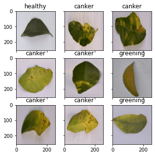
从加载图像到显示的完整代码如下。
from tensorflow.keras.utils import image_dataset_from_directory
import matplotlib.pyplot as plt

# use image_dataset_from_directory() to load images, with image size scaled to 256x256
PATH='.../Citrus/Leaves'  # modify to your path
ds = image_dataset_from_directory(PATH,
                                  validation_split=0.2, subset="training",
                                  image_size=(256,256), interpolation="mitchellcubic",
                                  crop_to_aspect_ratio=True,
                                  seed=42, shuffle=True, batch_size=32)

# Take one batch from dataset and display the images
fig, ax = plt.subplots(3, 3, sharex=True, sharey=True, figsize=(5,5))

for images, labels in ds.take(1):
    for i in range(3):
        for j in range(3):
            ax[i][j].imshow(images[i*3+j].numpy().astype("uint8"))
            ax[i][j].set_title(ds.class_names[labels[i*3+j]])
plt.show()
注意,如果你使用tensorflow_datasets 来获取图像,样本会以字典的形式呈现,而不是(image,label)的元组。你应该把你的代码稍微改变一下,变成下面的样子。
import tensorflow_datasets as tfds
import matplotlib.pyplot as plt

# use tfds.load() or image_dataset_from_directory() to load images
ds, meta = tfds.load('citrus_leaves', with_info=True, split='train', shuffle_files=True)
ds = ds.batch(32)

# Take one batch from dataset and display the images
fig, ax = plt.subplots(3, 3, sharex=True, sharey=True, figsize=(5,5))

for sample in ds.take(1):
    images, labels = sample["image"], sample["label"]
    for i in range(3):
        for j in range(3):
            ax[i][j].imshow(images[i*3+j].numpy().astype("uint8"))
            ax[i][j].set_title(meta.features['label'].int2str(labels[i*3+j]))
plt.show()
在这篇文章的其余部分,我们假设数据集是用image_dataset_from_directory() 创建的。如果你的数据集的创建方式不同,你可能需要稍微调整一下代码。
Keras的预处理层
Keras自带了许多神经网络层,比如我们需要训练的卷积层。还有一些没有参数的层需要训练,比如将图像等数组转换为矢量的扁平化层。
Keras中的预处理层是专门为在神经网络的早期阶段使用而设计的。我们可以用它们来进行图像预处理,比如调整图像的大小或旋转,或者调整亮度和对比度。虽然预处理层应该是更大的神经网络的一部分,但我们也可以将它们作为函数使用。下面是我们如何将调整大小层作为一个函数来转换一些图像,并将其与原始图像并排显示。
...

# create a resizing layer
out_height, out_width = 128,256
resize = tf.keras.layers.Resizing(out_height, out_width)

# show original vs resized
fig, ax = plt.subplots(2, 3, figsize=(6,4))

for images, labels in ds.take(1):
    for i in range(3):
        ax[0][i].imshow(images[i].numpy().astype("uint8"))
        ax[0][i].set_title("original")
        # resize
        ax[1][i].imshow(resize(images[i]).numpy().astype("uint8"))
        ax[1][i].set_title("resize")
plt.show()
我们的图像是256×256像素的,调整层将使它们变成256×128像素。上述代码的输出如下。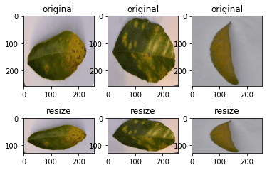
由于调整大小层本身是一个函数,我们可以将它们与数据集本身相连接。比如说。
...
def augment(image, label):
    return resize(image), label

resized_ds = ds.map(augment)

for image, label in resized_ds:
   ...
数据集ds ,其样本形式为(image, label) 。因此,我们创建了一个函数,接收这样的元组,用调整大小层对图像进行预处理。我们把这个函数作为数据集中map() 的参数。当我们从用map() 函数创建的新数据集中抽取样本时,图像将是一个经过转换的图像。
还有更多的预处理层可用。在下面,我们将演示一些。
正如我们上面看到的,我们可以调整图像的大小。我们还可以随机地放大或缩小图像的高度或宽度。同样地,我们可以放大或缩小图像。下面是一个例子,以各种方式操纵图像的大小,最多可增加或减少30%。
...

# Create preprocessing layers
out_height, out_width = 128,256
resize = tf.keras.layers.Resizing(out_height, out_width)
height = tf.keras.layers.RandomHeight(0.3)
width = tf.keras.layers.RandomWidth(0.3)
zoom = tf.keras.layers.RandomZoom(0.3)

# Visualize images and augmentations
fig, ax = plt.subplots(5, 3, figsize=(6,14))

for images, labels in ds.take(1):
    for i in range(3):
        ax[0][i].imshow(images[i].numpy().astype("uint8"))
        ax[0][i].set_title("original")
        # resize
        ax[1][i].imshow(resize(images[i]).numpy().astype("uint8"))
        ax[1][i].set_title("resize")
        # height
        ax[2][i].imshow(height(images[i]).numpy().astype("uint8"))
        ax[2][i].set_title("height")
        # width
        ax[3][i].imshow(width(images[i]).numpy().astype("uint8"))
        ax[3][i].set_title("width")
        # zoom
        ax[4][i].imshow(zoom(images[i]).numpy().astype("uint8"))
        ax[4][i].set_title("zoom")
plt.show()
这段代码显示的图像如下。
虽然我们在调整大小中指定了一个固定的尺寸,但在其他增强中我们有一个随机的操作量。
我们还可以使用预处理层进行翻转、旋转、裁剪和几何平移。
...
# Create preprocessing layers
flip = tf.keras.layers.RandomFlip("horizontal_and_vertical") # or "horizontal", "vertical"
rotate = tf.keras.layers.RandomRotation(0.2)
crop = tf.keras.layers.RandomCrop(out_height, out_width)
translation = tf.keras.layers.RandomTranslation(height_factor=0.2, width_factor=0.2)

# Visualize augmentations
fig, ax = plt.subplots(5, 3, figsize=(6,14))

for images, labels in ds.take(1):
    for i in range(3):
        ax[0][i].imshow(images[i].numpy().astype("uint8"))
        ax[0][i].set_title("original")
        # flip
        ax[1][i].imshow(flip(images[i]).numpy().astype("uint8"))
        ax[1][i].set_title("flip")
        # crop
        ax[2][i].imshow(crop(images[i]).numpy().astype("uint8"))
        ax[2][i].set_title("crop")
        # translation
        ax[3][i].imshow(translation(images[i]).numpy().astype("uint8"))
        ax[3][i].set_title("translation")
        # rotate
        ax[4][i].imshow(rotate(images[i]).numpy().astype("uint8"))
        ax[4][i].set_title("rotate")
plt.show()
这段代码显示了以下图像。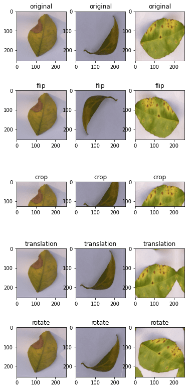
最后,我们也可以对颜色调整做增强处理。
...
brightness = tf.keras.layers.RandomBrightness([-0.8,0.8])
contrast = tf.keras.layers.RandomContrast(0.2)

# Visualize augmentation
fig, ax = plt.subplots(3, 3, figsize=(6,7))

for images, labels in ds.take(1):
    for i in range(3):
        ax[0][i].imshow(images[i].numpy().astype("uint8"))
        ax[0][i].set_title("original")
        # brightness
        ax[1][i].imshow(brightness(images[i]).numpy().astype("uint8"))
        ax[1][i].set_title("brightness")
        # contrast
        ax[2][i].imshow(contrast(images[i]).numpy().astype("uint8"))
        ax[2][i].set_title("contrast")
plt.show()
这显示的图像如下。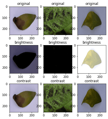
为了完整起见,下面是显示各种增强的结果的代码。
from tensorflow.keras.utils import image_dataset_from_directory
import tensorflow as tf
import matplotlib.pyplot as plt

# use image_dataset_from_directory() to load images, with image size scaled to 256x256
PATH='.../Citrus/Leaves'  # modify to your path
ds = image_dataset_from_directory(PATH,
                                  validation_split=0.2, subset="training",
                                  image_size=(256,256), interpolation="mitchellcubic",
                                  crop_to_aspect_ratio=True,
                                  seed=42, shuffle=True, batch_size=32)

# Create preprocessing layers
out_height, out_width = 128,256
resize = tf.keras.layers.Resizing(out_height, out_width)
height = tf.keras.layers.RandomHeight(0.3)
width = tf.keras.layers.RandomWidth(0.3)
zoom = tf.keras.layers.RandomZoom(0.3)

flip = tf.keras.layers.RandomFlip("horizontal_and_vertical")
rotate = tf.keras.layers.RandomRotation(0.2)
crop = tf.keras.layers.RandomCrop(out_height, out_width)
translation = tf.keras.layers.RandomTranslation(height_factor=0.2, width_factor=0.2)

brightness = tf.keras.layers.RandomBrightness([-0.8,0.8])
contrast = tf.keras.layers.RandomContrast(0.2)

# Visualize images and augmentations
fig, ax = plt.subplots(5, 3, figsize=(6,14))
for images, labels in ds.take(1):
    for i in range(3):
        ax[0][i].imshow(images[i].numpy().astype("uint8"))
        ax[0][i].set_title("original")
        # resize
        ax[1][i].imshow(resize(images[i]).numpy().astype("uint8"))
        ax[1][i].set_title("resize")
        # height
        ax[2][i].imshow(height(images[i]).numpy().astype("uint8"))
        ax[2][i].set_title("height")
        # width
        ax[3][i].imshow(width(images[i]).numpy().astype("uint8"))
        ax[3][i].set_title("width")
        # zoom
        ax[4][i].imshow(zoom(images[i]).numpy().astype("uint8"))
        ax[4][i].set_title("zoom")
plt.show()

fig, ax = plt.subplots(5, 3, figsize=(6,14))
for images, labels in ds.take(1):
    for i in range(3):
        ax[0][i].imshow(images[i].numpy().astype("uint8"))
        ax[0][i].set_title("original")
        # flip
        ax[1][i].imshow(flip(images[i]).numpy().astype("uint8"))
        ax[1][i].set_title("flip")
        # crop
        ax[2][i].imshow(crop(images[i]).numpy().astype("uint8"))
        ax[2][i].set_title("crop")
        # translation
        ax[3][i].imshow(translation(images[i]).numpy().astype("uint8"))
        ax[3][i].set_title("translation")
        # rotate
        ax[4][i].imshow(rotate(images[i]).numpy().astype("uint8"))
        ax[4][i].set_title("rotate")
plt.show()

fig, ax = plt.subplots(3, 3, figsize=(6,7))
for images, labels in ds.take(1):
    for i in range(3):
        ax[0][i].imshow(images[i].numpy().astype("uint8"))
        ax[0][i].set_title("original")
        # brightness
        ax[1][i].imshow(brightness(images[i]).numpy().astype("uint8"))
        ax[1][i].set_title("brightness")
        # contrast
        ax[2][i].imshow(contrast(images[i]).numpy().astype("uint8"))
        ax[2][i].set_title("contrast")
plt.show()
最后,需要指出的是,如果对输入图像进行缩放,大多数神经网络模型可以更好地工作。虽然我们通常使用8位无符号整数来表示图像中的像素值(例如,使用上述imshow() 来显示),但神经网络更喜欢像素值在0和1之间,或者在-1和+1之间。这也可以通过预处理层来完成。下面是我们如何更新上面的一个例子,将缩放层加入到增强中。
...
out_height, out_width = 128,256
resize = tf.keras.layers.Resizing(out_height, out_width)
rescale = tf.keras.layers.Rescaling(1/127.5, offset=-1)  # rescale pixel values to [-1,1]

def augment(image, label):
    return rescale(resize(image)), label

rescaled_resized_ds = ds.map(augment)

for image, label in rescaled_resized_ds:
   ...
使用tf.image API进行扩增
除了预处理层,tf.image 模块还提供了一些用于增强的功能。与预处理层不同的是,这些函数是为了在用户定义的函数中使用,并使用map() ,分配给数据集,正如我们在上面看到的。
tf.image 所提供的函数与预处理层并不重复,尽管有一些重叠的地方。下面是一个使用tf.image 的函数来调整图像大小和裁剪的例子。
...

fig, ax = plt.subplots(5, 3, figsize=(6,14))

for images, labels in ds.take(1):
    for i in range(3):
        # original
        ax[0][i].imshow(images[i].numpy().astype("uint8"))
        ax[0][i].set_title("original")
        # resize
        h = int(256 * tf.random.uniform([], minval=0.8, maxval=1.2))
        w = int(256 * tf.random.uniform([], minval=0.8, maxval=1.2))
        ax[1][i].imshow(tf.image.resize(images[i], [h,w]).numpy().astype("uint8"))
        ax[1][i].set_title("resize")
        # crop
        y, x, h, w = (128 * tf.random.uniform((4,))).numpy().astype("uint8")
        ax[2][i].imshow(tf.image.crop_to_bounding_box(images[i], y, x, h, w).numpy().astype("uint8"))
        ax[2][i].set_title("crop")
        # central crop
        x = tf.random.uniform([], minval=0.4, maxval=1.0)
        ax[3][i].imshow(tf.image.central_crop(images[i], x).numpy().astype("uint8"))
        ax[3][i].set_title("central crop")
        # crop to (h,w) at random offset
        h, w = (256 * tf.random.uniform((2,))).numpy().astype("uint8")
        seed = tf.random.uniform((2,), minval=0, maxval=65536).numpy().astype("int32")
        ax[4][i].imshow(tf.image.stateless_random_crop(images[i], [h,w,3], seed).numpy().astype("uint8"))
        ax[4][i].set_title("random crop")
plt.show()
下面是上述代码的输出。
虽然图像的显示符合我们对代码的期望,但tf.image 函数的使用与预处理层的使用有很大不同。每个tf.image 函数都是不同的。因此,我们可以看到crop_to_bounding_box() 函数需要像素坐标,但central_crop() 函数则假定分数比作为参数。
这些函数在处理随机性的方式上也不同。其中一些函数并不假设随机行为。因此,随机调整大小应该在调用调整大小函数之前,用随机数发生器单独生成准确的输出大小。其他一些函数,如stateless_random_crop() ,可以进行随机增殖,但需要明确指定int32 中的一对随机种子。
为了继续这个例子,还有翻转图像和提取Sobel边缘的函数。
...
fig, ax = plt.subplots(5, 3, figsize=(6,14))

for images, labels in ds.take(1):
    for i in range(3):
        ax[0][i].imshow(images[i].numpy().astype("uint8"))
        ax[0][i].set_title("original")
        # flip
        seed = tf.random.uniform((2,), minval=0, maxval=65536).numpy().astype("int32")
        ax[1][i].imshow(tf.image.stateless_random_flip_left_right(images[i], seed).numpy().astype("uint8"))
        ax[1][i].set_title("flip left-right")
        # flip
        seed = tf.random.uniform((2,), minval=0, maxval=65536).numpy().astype("int32")
        ax[2][i].imshow(tf.image.stateless_random_flip_up_down(images[i], seed).numpy().astype("uint8"))
        ax[2][i].set_title("flip up-down")
        # sobel edge
        sobel = tf.image.sobel_edges(images[i:i+1])
        ax[3][i].imshow(sobel[0, ..., 0].numpy().astype("uint8"))
        ax[3][i].set_title("sobel y")
        # sobel edge
        ax[4][i].imshow(sobel[0, ..., 1].numpy().astype("uint8"))
        ax[4][i].set_title("sobel x")
plt.show()
其中显示如下。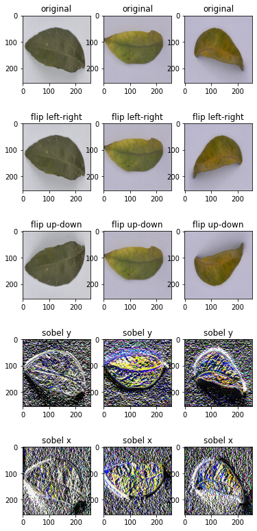
还有以下是操作亮度、对比度和颜色的函数。
...
fig, ax = plt.subplots(5, 3, figsize=(6,14))

for images, labels in ds.take(1):
    for i in range(3):
        ax[0][i].imshow(images[i].numpy().astype("uint8"))
        ax[0][i].set_title("original")
        # brightness
        seed = tf.random.uniform((2,), minval=0, maxval=65536).numpy().astype("int32")
        ax[1][i].imshow(tf.image.stateless_random_brightness(images[i], 0.3, seed).numpy().astype("uint8"))
        ax[1][i].set_title("brightness")
        # contrast
        ax[2][i].imshow(tf.image.stateless_random_contrast(images[i], 0.7, 1.3, seed).numpy().astype("uint8"))
        ax[2][i].set_title("contrast")
        # saturation
        ax[3][i].imshow(tf.image.stateless_random_saturation(images[i], 0.7, 1.3, seed).numpy().astype("uint8"))
        ax[3][i].set_title("saturation")
        # hue
        ax[4][i].imshow(tf.image.stateless_random_hue(images[i], 0.3, seed).numpy().astype("uint8"))
        ax[4][i].set_title("hue")
plt.show()
这段代码显示如下。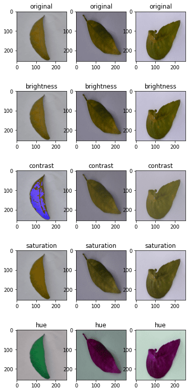
下面是显示上述所有内容的完整代码。
from tensorflow.keras.utils import image_dataset_from_directory
import tensorflow as tf
import matplotlib.pyplot as plt

# use image_dataset_from_directory() to load images, with image size scaled to 256x256
PATH='.../Citrus/Leaves'  # modify to your path
ds = image_dataset_from_directory(PATH,
                                  validation_split=0.2, subset="training",
                                  image_size=(256,256), interpolation="mitchellcubic",
                                  crop_to_aspect_ratio=True,
                                  seed=42, shuffle=True, batch_size=32)

# Visualize tf.image augmentations

fig, ax = plt.subplots(5, 3, figsize=(6,14))
for images, labels in ds.take(1):
    for i in range(3):
        # original
        ax[0][i].imshow(images[i].numpy().astype("uint8"))
        ax[0][i].set_title("original")
        # resize
        h = int(256 * tf.random.uniform([], minval=0.8, maxval=1.2))
        w = int(256 * tf.random.uniform([], minval=0.8, maxval=1.2))
        ax[1][i].imshow(tf.image.resize(images[i], [h,w]).numpy().astype("uint8"))
        ax[1][i].set_title("resize")
        # crop
        y, x, h, w = (128 * tf.random.uniform((4,))).numpy().astype("uint8")
        ax[2][i].imshow(tf.image.crop_to_bounding_box(images[i], y, x, h, w).numpy().astype("uint8"))
        ax[2][i].set_title("crop")
        # central crop
        x = tf.random.uniform([], minval=0.4, maxval=1.0)
        ax[3][i].imshow(tf.image.central_crop(images[i], x).numpy().astype("uint8"))
        ax[3][i].set_title("central crop")
        # crop to (h,w) at random offset
        h, w = (256 * tf.random.uniform((2,))).numpy().astype("uint8")
        seed = tf.random.uniform((2,), minval=0, maxval=65536).numpy().astype("int32")
        ax[4][i].imshow(tf.image.stateless_random_crop(images[i], [h,w,3], seed).numpy().astype("uint8"))
        ax[4][i].set_title("random crop")
plt.show()

fig, ax = plt.subplots(5, 3, figsize=(6,14))
for images, labels in ds.take(1):
    for i in range(3):
        ax[0][i].imshow(images[i].numpy().astype("uint8"))
        ax[0][i].set_title("original")
        # flip
        seed = tf.random.uniform((2,), minval=0, maxval=65536).numpy().astype("int32")
        ax[1][i].imshow(tf.image.stateless_random_flip_left_right(images[i], seed).numpy().astype("uint8"))
        ax[1][i].set_title("flip left-right")
        # flip
        seed = tf.random.uniform((2,), minval=0, maxval=65536).numpy().astype("int32")
        ax[2][i].imshow(tf.image.stateless_random_flip_up_down(images[i], seed).numpy().astype("uint8"))
        ax[2][i].set_title("flip up-down")
        # sobel edge
        sobel = tf.image.sobel_edges(images[i:i+1])
        ax[3][i].imshow(sobel[0, ..., 0].numpy().astype("uint8"))
        ax[3][i].set_title("sobel y")
        # sobel edge
        ax[4][i].imshow(sobel[0, ..., 1].numpy().astype("uint8"))
        ax[4][i].set_title("sobel x")
plt.show()

fig, ax = plt.subplots(5, 3, figsize=(6,14))
for images, labels in ds.take(1):
    for i in range(3):
        ax[0][i].imshow(images[i].numpy().astype("uint8"))
        ax[0][i].set_title("original")
        # brightness
        seed = tf.random.uniform((2,), minval=0, maxval=65536).numpy().astype("int32")
        ax[1][i].imshow(tf.image.stateless_random_brightness(images[i], 0.3, seed).numpy().astype("uint8"))
        ax[1][i].set_title("brightness")
        # contrast
        ax[2][i].imshow(tf.image.stateless_random_contrast(images[i], 0.7, 1.3, seed).numpy().astype("uint8"))
        ax[2][i].set_title("contrast")
        # saturation
        ax[3][i].imshow(tf.image.stateless_random_saturation(images[i], 0.7, 1.3, seed).numpy().astype("uint8"))
        ax[3][i].set_title("saturation")
        # hue
        ax[4][i].imshow(tf.image.stateless_random_hue(images[i], 0.3, seed).numpy().astype("uint8"))
        ax[4][i].set_title("hue")
plt.show()
这些增强功能对于大多数使用来说应该是足够的。但如果你有一些关于增强的具体想法,可能你会需要一个更好的图像处理库。OpenCV和Pillow是常见但功能强大的库,可以让你更好地转换图像。
在神经网络中使用预处理层
我们在上面的例子中把Keras的预处理层作为函数使用。但它们也可以作为神经网络中的层使用。它的使用很微妙。下面是一个例子,说明我们如何将预处理层纳入分类网络,并使用数据集对其进行训练。
from tensorflow.keras.utils import image_dataset_from_directory
import tensorflow as tf
import matplotlib.pyplot as plt

# use image_dataset_from_directory() to load images, with image size scaled to 256x256
PATH='.../Citrus/Leaves'  # modify to your path
ds = image_dataset_from_directory(PATH,
                                  validation_split=0.2, subset="training",
                                  image_size=(256,256), interpolation="mitchellcubic",
                                  crop_to_aspect_ratio=True,
                                  seed=42, shuffle=True, batch_size=32)

AUTOTUNE = tf.data.AUTOTUNE
ds = ds.cache().prefetch(buffer_size=AUTOTUNE)

num_classes = 5
model = tf.keras.Sequential([
  tf.keras.layers.RandomFlip("horizontal_and_vertical"),
  tf.keras.layers.RandomRotation(0.2),
  tf.keras.layers.Rescaling(1/127.0, offset=-1),
  tf.keras.layers.Conv2D(32, 3, activation='relu'),
  tf.keras.layers.MaxPooling2D(),
  tf.keras.layers.Conv2D(32, 3, activation='relu'),
  tf.keras.layers.MaxPooling2D(),
  tf.keras.layers.Conv2D(32, 3, activation='relu'),
  tf.keras.layers.MaxPooling2D(),
  tf.keras.layers.Flatten(),
  tf.keras.layers.Dense(128, activation='relu'),
  tf.keras.layers.Dense(num_classes)
])

model.compile(optimizer='adam',
              loss=tf.keras.losses.SparseCategoricalCrossentropy(from_logits=True),
              metrics=['accuracy'])

model.fit(ds, epochs=3)
运行这段代码可以得到以下输出。
Found 609 files belonging to 5 classes.
Using 488 files for training.
Epoch 1/3
16/16 [==============================] - 5s 253ms/step - loss: 1.4114 - accuracy: 0.4283
Epoch 2/3
16/16 [==============================] - 4s 259ms/step - loss: 0.8101 - accuracy: 0.6475
Epoch 3/3
16/16 [==============================] - 4s 267ms/step - loss: 0.7015 - accuracy: 0.7111
在上面的代码中,我们用cache() 和prefetch() 创建了数据集。这是一种性能技术,允许数据集在神经网络训练时异步地准备数据。如果数据集有一些使用map() 函数分配的其他增强,这将是非常重要的。
如果你去掉了RandomFlip 和RandomRotation 层,你会看到准确率有一些提高,因为你使问题变得更容易。然而,由于我们希望网络能够在广泛的图像质量和属性的变化上有良好的预测,使用增强可以帮助我们产生的网络更加强大。
进一步阅读
以下是TensorFlow中与上述例子相关的文档。
摘要
在这篇文章中,你已经看到了我们如何使用tf.data 数据集与Keras和TensorFlow的图像增强功能。
具体来说,你学到了:
- 如何使用Keras的预处理层,无论是作为一个函数还是作为神经网络的一部分
- 如何创建你自己的图像增强函数,并使用
map()函数将其应用到数据集上 - 如何使用
tf.image模块提供的函数进行图像增强
