

简介
在这篇文章中,我们将带你了解使用ggplot2的Heatmap教程,ggplot2是一个常用的包,用于在R中创建漂亮的可视化。我们将首先了解语法,然后看到不同类型的使用ggplot2的Heatmap例子。
ggplot2中热图的语法
在ggplot2中生成热图的最小语法是
ggplot(, mapping = aes())+ geom_tile()
我们还可以通过添加更多的图层来定制热图,如主题、实验室等。
R语言中使用ggplot2绘制热图的例子
准备数据集
在ggplot2中的所有热图例子中,我们将使用 "heart.csv "数据集。
转换成一个叫做df的数据框
In[2]:
df <- read.table("heart.csv",header=TRUE,sep=',')
head(df)
输出[2]:
| ï...年龄 | 性别 | cp | trestbps | chol | fbs | 补钙 | タルチャー | 准确 | 老峰 | 坡度 | ca | 峰值 | 目标 |
|---|---|---|---|---|---|---|---|---|---|---|---|---|---|
| 63 | 1 | 3 | 145 | 233 | 1 | 0 | 150 | 0 | 2.3 | 0 | 0 | 1 | 1 |
| 37 | 1 | 2 | 130 | 250 | 0 | 1 | 187 | 0 | 3.5 | 0 | 0 | 2 | 1 |
| 41 | 0 | 1 | 130 | 204 | 0 | 0 | 172 | 0 | 1.4 | 2 | 0 | 2 | 1 |
| 56 | 1 | 1 | 120 | 236 | 0 | 1 | 178 | 0 | 0.8 | 2 | 0 | 2 | 1 |
| 57 | 0 | 0 | 120 | 354 | 0 | 1 | 163 | 1 | 0.6 | 2 | 0 | 2 | 1 |
| 57 | 1 | 0 | 140 | 192 | 0 | 1 | 148 | 0 | 0.4 | 1 | 0 | 1 | 1 |
我们使用cor()函数来计算两个向量之间的相关性,这又为我们生成了一个数据集的相关矩阵
In[3]:
cormat <- round(cor(df),2)
head(cormat)
Out[3]:
| ï...年龄 | 性别 | cp | trestbps | chol | fbs | 补钙 | 钍 | ǞǞǞ | 老峰 | 坡度 | ca | thal | 目标 | |
|---|---|---|---|---|---|---|---|---|---|---|---|---|---|---|
| ï...年龄 | 1.00 | -0.10 | -0.07 | 0.28 | 0.21 | 0.12 | -0.12 | -0.40 | 0.10 | 0.21 | -0.17 | 0.28 | 0.07 | -0.23 |
| 性别 | -0.10 | 1.00 | -0.05 | -0.06 | -0.20 | 0.05 | -0.06 | -0.04 | 0.14 | 0.10 | -0.03 | 0.12 | 0.21 | -0.28 |
| cp | -0.07 | -0.05 | 1.00 | 0.05 | -0.08 | 0.09 | 0.04 | 0.30 | -0.39 | -0.15 | 0.12 | -0.18 | -0.16 | 0.43 |
| 栈桥 | 0.28 | -0.06 | 0.05 | 1.00 | 0.12 | 0.18 | -0.11 | -0.05 | 0.07 | 0.19 | -0.12 | 0.10 | 0.06 | -0.14 |
| 胆汁 | 0.21 | -0.20 | -0.08 | 0.12 | 1.00 | 0.01 | -0.15 | -0.01 | 0.07 | 0.05 | 0.00 | 0.07 | 0.10 | -0.09 |
| fbs | 0.12 | 0.05 | 0.09 | 0.18 | 0.01 | 1.00 | -0.08 | -0.01 | 0.03 | 0.01 | -0.06 | 0.14 | -0.03 | -0.03 |
使用reshape2库,我们随后可以使用melt函数将我们的数据框转换成长格式,并拉伸数据框。这个转换后的数据集将在随后的所有例子中使用。
In[3]:
library(reshape2)
melted_cormat <- melt(cormat)
head(melted_cormat)
Out[3]:
| Var1 | Var2 | 价值 |
|---|---|---|
| ï...年龄 | ï...年龄 | 1.00 |
| 性别 | ï...年龄 | -0.10 |
| cp | ï...年龄 | -0.07 |
| trestbps | ï...年龄 | 0.28 |
| chol | ï...年龄 | 0.21 |
| 脂肪细胞 | ï...年龄 | 0.12 |
加载ggplot2
首先,让我们加载ggplot2库,如下图所示:
在[4]中。
library(ggplot2)
例1:ggplot2中的基本热图
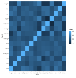
ggplot2中的基本热力图是通过使用geom_tile()层创建的,如下面的例子所示。
在[5]中。
ggplot(data = melted_cormat, aes(x=Var1, y=Var2, fill=value)) +
  geom_tile()
Out[5]:
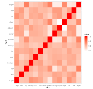
例2:热力图中的梯度填充(Scale_fill_gradient)功能
Scale_fill_gradient用于在热力图中添加颜色梯度。它有两个参数,即高和低,用于指定梯度比例。
In[6]:
ggplot(data=melted_cormat,aes(x = Var1, y = Var2, fill = value))+
geom_tile()+scale_fill_gradient(high = "red", low = "white")
输出[6]:
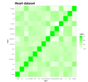
例3:给热力图添加标题
让我们给我们的热力图添加一个标题,给它更多的描述。我们可以通过使用ggtitle()来做到这一点。
在[7]中:
ggplot(data=melted_cormat,aes(x = Var1, y = Var2, fill = value))+
geom_tile()+scale_fill_gradient(high = "green", low = "white") +
ggtitle("Heart dataset")+ theme(plot.title = element_text(size = 20, face = "bold"))
Out[7]:
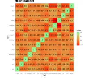
例4:用热力图可视化相关关系
这里的每个单元格都描述了相交变量之间的关系,比如说线性相关。这个图可以帮助分析人员了解变量之间的关系,同时描述性或预测性的统计模型。
In[8]:
ggplot(data=melted_cormat,aes(x = Var1, y = Var2, fill = value))+
geom_tile()+scale_fill_gradient(high = "green", low = "red")+
ggtitle("Heart dataset")+
theme(plot.title = element_text(size = 20, face = "bold"))+
geom_text(aes(label = round(value, 3)))+
scale_fill_continuous(low = "red", high = "lightgreen")
Out[8]:
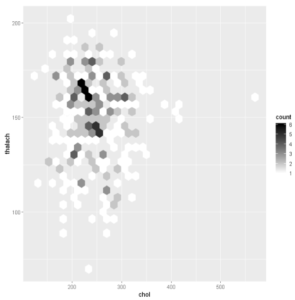
例5:六边形图
添加六边形绑定 函数geom_hex()产生一个带有六边形绑定的散点图。hexbin R包是进行六边形划分的必要条件。如果你没有这个包,可以使用下面的R代码,用require(hexbin)来安装。
在[9]:
# Default plot
ggplot(df,aes(chol,thalach))+ geom_hex()
# Change the number of bins
ggplot(df,aes(chol,thalach)) + geom_hex(bins = 10)
输出[9]:
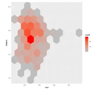
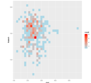
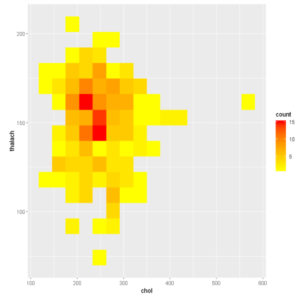
例6:添加2d bin计数的热图
函数geom_bin2d()产生一个带有矩形仓的散点图。每个bin中的观测值被计算出来,并以热图的形式显示。
In[10]:
# Default plot
ggplot(df,aes(chol,thalach)) + geom_bin2d()
# Change the number of bins
ggplot(df,aes(chol,thalach)) + geom_bin2d(bins = 15)
Out[10]:
- 还可以阅读 - Python中的热图 Matplotlib
- 还读了 - Python Seaborn中的热图
