鸣叫 鸣叫 分享 分享
为支持向量机(SVM)分类器提供动力的数学是美丽的。重要的是,不仅要学习SVM的基本模型,还要知道如何从头开始实现整个模型。这是我们关于SVM的系列教程的继续。在这个系列的第一部分和第二部分,我们讨论了线性SVM背后的数学模型。在本教程中,我们将展示如何使用Python的SciPy库所提供的优化例程来构建一个SVM线性分类器。
完成本教程后,你将知道。
- 如何使用 SciPy 的优化例程
- 如何定义目标函数
- 如何定义边界和线性约束
- 如何在Python中实现你自己的SVM分类器
让我们开始吧。

拉格朗日乘法的方法。支持向量机背后的理论(第三部分:在Python中从头开始实现SVM)
Sculpture Gyre by Thomas Sayre, Photo by Mehreen Saeed, some rights reserved.
教程概述
本教程分为两部分;它们是:。
- SVM的优化问题
- Python中的优化问题解决方案
- 定义目标函数
- 定义边界和线性约束
- 用不同的C值解决该问题
前提条件
在本教程中,我们假定你已经熟悉了以下主题。你可以点击个别链接以获得更多细节。
符号和假设
一个基本的SVM机器假设是一个二进制分类问题。假设我们有m的训练点,每个点都是一个n的维向量。我们将使用以下符号。
- m:训练点总数
- n:每个训练点的维度
- x:数据点,是一个n维度的向量
- i:用来索引训练点的下标。0/leqi<m
- k:用来索引训练点的下标。0leqk<m
- j:用来索引训练点的每个维度的下标
- t:一个数据点的标签。它是一个m维的向量,t_iin−1,+1
- T:转置运算符
- w:表示超平面系数的权重向量。它也是一个n维的向量
- alpha。拉格朗日乘数的矢量,也是一个m维的矢量
- C:用户定义的惩罚因子/规范化常数
SVM的优化问题
SVM分类器最大化以下拉格朗日对偶:
L_d=−frac12.L_d=−sum_i/sum_k/alpha_i/alpha_kt_it_k(x_i)T(x_k)+sˋum_i/alpha_i
上述函数受制于以下约束。
\begin{eqnarray}
0 \leq \alpha_i \leq C, & \forall i\
\sum_i \alpha_i t_i = 0& \
end{eqnarray} 。
我们所要做的就是找到与每个训练点相关的拉格朗日乘数alpha,同时满足上述约束。
SVM的Python实现
我们将使用SciPy优化包来找到拉格朗日乘数的最优值,并计算软边际和分离超平面。
导入部分和常量
我们来写一下优化、绘图和合成数据生成的导入部分。
import numpy as np
from scipy.optimize import Bounds, BFGS
from scipy.optimize import LinearConstraint, minimize
import matplotlib.pyplot as plt
import seaborn as sns
import sklearn.datasets as dt
我们还需要以下常数来检测所有数值接近零的字母,所以我们需要定义我们自己的零的阈值。
ZERO = 1e-7
定义数据点和标签
让我们定义一个非常简单的数据集,相应的标签和一个简单的程序来绘制这个数据。可以选择的是,如果给绘图函数一串字母,那么它也会给所有支持向量贴上相应的字母值。请记住,支持向量是那些alpha>0的点。
dat = np.array([[0, 3], [-1, 0], [1, 2], [2, 1], [3,3], [0, 0], [-1, -1], [-3, 1], [3, 1]])
labels = np.array([1, 1, 1, 1, 1, -1, -1, -1, -1])
def plot_x(x, t, alpha=[], C=0):
sns.scatterplot(dat[:,0], dat[:, 1], style=labels,
hue=labels, markers=['s', 'P'],
palette=['magenta', 'green'])
if len(alpha) > 0:
alpha_str = np.char.mod('%.1f', np.round(alpha, 1))
ind_sv = np.where(alpha > ZERO)[0]
for i in ind_sv:
plt.gca().text(dat[i,0], dat[i, 1]-.25, alpha_str[i] )
plot_x(dat, labels)

minimize() 函数
让我们看一下scipy.optimize 库中的minimize() 函数。它需要以下参数。
- 要最小化的目标函数。在我们的例子中是拉格朗日对偶。
- 最小化所涉及的变量的初始值。在这个问题中,我们必须确定拉格朗日乘数alpha。我们将随机地初始化所有alpha。
- 用来进行优化的方法。我们将使用
trust-constr 。
- 对alpha的线性约束。
- alpha的界限。
定义目标函数
我们的目标函数是上面定义的L_d,它必须被最大化。由于我们使用的是minimize() ,我们必须用L_d乘以(-1)来最大化它。其实现方法如下。目标函数的第一个参数是进行优化的变量。我们还需要训练点和相应的标签作为附加参数。
你可以通过使用矩阵来缩短下面给出的lagrange_dual() 函数的代码。然而,在本教程中,为了使一切都清晰明了,它保持得非常简单。
def lagrange_dual(alpha, x, t):
result = 0
ind_sv = np.where(alpha > ZERO)[0]
for i in ind_sv:
for k in ind_sv:
result = result + alpha[i]*alpha[k]*t[i]*t[k]*np.dot(x[i, :], x[k, :])
result = 0.5*result - sum(alpha)
return result
定义线性约束
每个点的阿尔法的线性约束由以下方式给出。
$
\sum_i \alpha_i t_i = 0
我们也可以写成:
\alpha_0 t_0 + \alpha_1 t_1 + \ldots \alpha_m t_m = 0
`LinearConstraint()` 方法要求将所有的约束条件写成矩阵形式,也就是。
\\begin{equation}
0 =
/begin{bmatrix}
t\_0 & t\_1 & \\ldots t\_m
/end{bmatrix}
/begin{bmatrix}
\\alpha\_0\\ \\alpha\_1\\ \\vdots \\ \\alpha\_m
/end{bmatrix}
\= 0
/end{equation} 。
第一个矩阵是`LinearConstraint()` 方法中的第一个参数。左边和右边的边界是第二个和第三个参数。
```
linear_constraint = LinearConstraint(labels, [0], [0])
print(linear_constraint)
```
```
<scipy.optimize._constraints.LinearConstraint object at 0x12c87f5b0>
```
### 界限的定义
alpha的边界是用`Bounds()` 方法定义的。所有字母都被限制在0和$C$之间。下面是一个$C=10$的例子。
```
bounds_alpha = Bounds(np.zeros(dat.shape[0]), np.full(dat.shape[0], 10))
print(bounds_alpha)
```
```
Bounds(array([0., 0., 0., 0., 0., 0., 0., 0., 0.]), array([10, 10, 10, 10, 10, 10, 10, 10, 10]))
```
### 定义查找字母的函数
让我们来写一个整体的程序,当给定参数`x`,`t`, 和`C` 时,找到`alpha` 的最佳值。目标函数需要额外的参数`x` 和`t` ,这些参数通过`minimize()` 中的args传递。
```
def optimize_alpha(x, t, C):
m, n = x.shape
np.random.seed(1)
# Initialize alphas to random values
alpha_0 = np.random.rand(m)*C
# Define the constraint
linear_constraint = LinearConstraint(t, [0], [0])
# Define the bounds
bounds_alpha = Bounds(np.zeros(m), np.full(m, C))
# Find the optimal value of alpha
result = minimize(lagrange_dual, alpha_0, args = (x, t), method='trust-constr',
hess=BFGS(), constraints=[linear_constraint],
bounds=bounds_alpha)
# The optimized value of alpha lies in result.x
alpha = result.x
return alpha
```
### 确定超平面
超平面的表达式为:
w^T x + w_0 = 0
对于超平面,我们需要权重向量$w$和常数$w\_0$。权重向量由以下公式给出:
w = \sum_i \alpha_i t_i x_i
如果有太多的训练点,最好只使用$alpha>0$的支持向量来计算权重向量。
对于$w\_0$,我们将从每个支持向量$s$中计算它,对于$alpha\_s < C$,然后取平均值。对于单个支持向量$x\_s$,$w\_0$由以下公式给出。
$
w\_0 = t\_s - w^T x\_s
一个支持向量的α不可能在数值上完全等于C。因此,我们可以从C中减去一个小常数,以找到所有支持向量的alpha_s<C。这是在get_w0() 函数中完成的。
def get_w(alpha, t, x):
m = len(x)
w = np.zeros(x.shape[1])
for i in range(m):
w = w + alpha[i]*t[i]*x[i, :]
return w
def get_w0(alpha, t, x, w, C):
C_numeric = C-ZERO
ind_sv = np.where((alpha > ZERO)&(alpha < C_numeric))[0]
w0 = 0.0
for s in ind_sv:
w0 = w0 + t[s] - np.dot(x[s, :], w)
w0 = w0 / len(ind_sv)
return w0
对测试点进行分类
为了对测试点x_test进行分类,我们使用y(x_test)的符号作为。
$
\text{label}_{x_{test}} = \text{sign}(y(x_{test})) = \text{sign}(w^T x_{test} + w_0)
让我们写出相应的函数,它可以把测试点的数组以及$w$和$w\_0$作为参数,对各种点进行分类。我们还添加了第二个函数来计算错误分类率。
```
def classify_points(x_test, w, w0):
# get y(x_test)
predicted_labels = np.sum(x_test*w, axis=1) + w0
predicted_labels = np.sign(predicted_labels)
# Assign a label arbitrarily a +1 if it is zero
predicted_labels[predicted_labels==0] = 1
return predicted_labels
def misclassification_rate(labels, predictions):
total = len(labels)
errors = sum(labels != predictions)
return errors/total*100
```
### 绘制边距和超平面
让我们也定义一些函数来绘制超平面和软边际。
```
def plot_hyperplane(w, w0):
x_coord = np.array(plt.gca().get_xlim())
y_coord = -w0/w[1] - w[0]/w[1] * x_coord
plt.plot(x_coord, y_coord, color='red')
def plot_margin(w, w0):
x_coord = np.array(plt.gca().get_xlim())
ypos_coord = 1/w[1] - w0/w[1] - w[0]/w[1] * x_coord
plt.plot(x_coord, ypos_coord, '--', color='green')
yneg_coord = -1/w[1] - w0/w[1] - w[0]/w[1] * x_coord
plt.plot(x_coord, yneg_coord, '--', color='magenta')
```
给SVM加电
------
现在是运行SVM的时候了。函数`display_SVM_result()` 将帮助我们可视化一切。我们将把α初始化为随机值,定义C并在这个函数中找到α的最佳值。我们还将绘制超平面、边际和数据点。支持向量也将由其相应的α值来标示。该图的标题将是错误的百分比和支持向量的数量。
```
def display_SVM_result(x, t, C):
# Get the alphas
alpha = optimize_alpha(x, t, C)
# Get the weights
w = get_w(alpha, t, x)
w0 = get_w0(alpha, t, x, w, C)
plot_x(x, t, alpha, C)
xlim = plt.gca().get_xlim()
ylim = plt.gca().get_ylim()
plot_hyperplane(w, w0)
plot_margin(w, w0)
plt.xlim(xlim)
plt.ylim(ylim)
# Get the misclassification error and display it as title
predictions = classify_points(x, w, w0)
err = misclassification_rate(t, predictions)
title = 'C = ' + str(C) + ', Errors: ' + '{:.1f}'.format(err) + '%'
title = title + ', total SV = ' + str(len(alpha[alpha > ZERO]))
plt.title(title)
display_SVM_result(dat, labels, 100)
plt.show()
```
[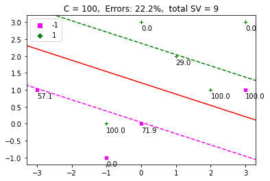](https://machinelearningmastery.com/wp-content/uploads/2021/12/svm2.png)
的影响`C`
------
如果你把`C` 的值改为 $\\infty$ ,那么软边距就变成了硬边距,对错误没有容忍度。在这种情况下,我们上面定义的问题是无法解决的。让我们生成一个人工点集,看看`C` 对分类的影响。为了理解整个问题,我们将使用一个简单的数据集,其中正面和负面的例子是可以分开的。
下面是通过`make_blobs()` 产生的点。
```
dat, labels = dt.make_blobs(n_samples=[20,20],
cluster_std=1,
random_state=0)
labels[labels==0] = -1
plot_x(dat, labels)
```
[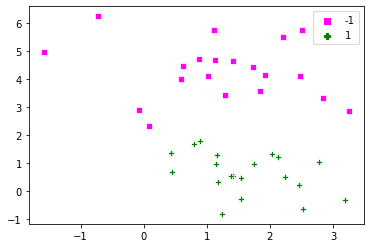](https://machinelearningmastery.com/wp-content/uploads/2021/12/svm3.png)
现在让我们定义不同的C值并运行代码。
```
fig = plt.figure(figsize=(8,25))
i=0
C_array = [1e-2, 100, 1e5]
for C in C_array:
fig.add_subplot(311+i)
display_SVM_result(dat, labels, C)
i = i + 1
```
### [](https://machinelearningmastery.com/wp-content/uploads/2021/12/svm4.png)对结果的评论
上面是一个很好的例子,它表明增加$C$,就会减少幅度。C$的高值对错误的惩罚更严格。较小的值允许更宽的余量和更多的误分类误差。因此,$C$定义了保证金最大化和分类错误之间的权衡。
综合代码
----
这里是合并后的代码,你可以把它粘贴到你的Python文件中并在你的终端运行。你可以用不同的$C$值进行实验,并尝试不同的优化方法,作为`minimize()` 函数的参数。
```
import numpy as np
# For optimization
from scipy.optimize import Bounds, BFGS
from scipy.optimize import LinearConstraint, minimize
# For plotting
import matplotlib.pyplot as plt
import seaborn as sns
# For generating dataset
import sklearn.datasets as dt
ZERO = 1e-7
def plot_x(x, t, alpha=[], C=0):
sns.scatterplot(dat[:,0], dat[:, 1], style=labels,
hue=labels, markers=['s', 'P'],
palette=['magenta', 'green'])
if len(alpha) > 0:
alpha_str = np.char.mod('%.1f', np.round(alpha, 1))
ind_sv = np.where(alpha > ZERO)[0]
for i in ind_sv:
plt.gca().text(dat[i,0], dat[i, 1]-.25, alpha_str[i] )
# Objective function
def lagrange_dual(alpha, x, t):
    result = 0
    ind_sv = np.where(alpha > ZERO)[0]
    for i in ind_sv:
        for k in ind_sv:
            result = result + alpha[i]*alpha[k]*t[i]*t[k]*np.dot(x[i, :], x[k, :])
    result = 0.5*result - sum(alpha)
    return result
def optimize_alpha(x, t, C):
m, n = x.shape
np.random.seed(1)
# Initialize alphas to random values
alpha_0 = np.random.rand(m)*C
# Define the constraint
linear_constraint = LinearConstraint(t, [0], [0])
# Define the bounds
bounds_alpha = Bounds(np.zeros(m), np.full(m, C))
# Find the optimal value of alpha
result = minimize(lagrange_dual, alpha_0, args = (x, t), method='trust-constr',
hess=BFGS(), constraints=[linear_constraint],
bounds=bounds_alpha)
# The optimized value of alpha lies in result.x
alpha = result.x
return alpha
def get_w(alpha, t, x):
    m = len(x)
    # Get all support vectors
    w = np.zeros(x.shape[1])
    for i in range(m):
        w = w + alpha[i]*t[i]*x[i, :]
    return w

def get_w0(alpha, t, x, w, C):
    C_numeric = C-ZERO
    # Indices of support vectors with alpha<C
    ind_sv = np.where((alpha > ZERO)&(alpha < C_numeric))[0]
    w0 = 0.0
    for s in ind_sv:
        w0 = w0 + t[s] - np.dot(x[s, :], w)
    # Take the average
    w0 = w0 / len(ind_sv)
    return w0
def classify_points(x_test, w, w0):
# get y(x_test)
predicted_labels = np.sum(x_test*w, axis=1) + w0
predicted_labels = np.sign(predicted_labels)
# Assign a label arbitrarily a +1 if it is zero
predicted_labels[predicted_labels==0] = 1
return predicted_labels
def misclassification_rate(labels, predictions):
total = len(labels)
errors = sum(labels != predictions)
return errors/total*100
def plot_hyperplane(w, w0):
x_coord = np.array(plt.gca().get_xlim())
y_coord = -w0/w[1] - w[0]/w[1] * x_coord
plt.plot(x_coord, y_coord, color='red')
def plot_margin(w, w0):
x_coord = np.array(plt.gca().get_xlim())
ypos_coord = 1/w[1] - w0/w[1] - w[0]/w[1] * x_coord
plt.plot(x_coord, ypos_coord, '--', color='green')
yneg_coord = -1/w[1] - w0/w[1] - w[0]/w[1] * x_coord
plt.plot(x_coord, yneg_coord, '--', color='magenta')
def display_SVM_result(x, t, C):
# Get the alphas
alpha = optimize_alpha(x, t, C)
# Get the weights
w = get_w(alpha, t, x)
w0 = get_w0(alpha, t, x, w, C)
plot_x(x, t, alpha, C)
xlim = plt.gca().get_xlim()
ylim = plt.gca().get_ylim()
plot_hyperplane(w, w0)
plot_margin(w, w0)
plt.xlim(xlim)
plt.ylim(ylim)
# Get the misclassification error and display it as title
predictions = classify_points(x, w, w0)
err = misclassification_rate(t, predictions)
title = 'C = ' + str(C) + ', Errors: ' + '{:.1f}'.format(err) + '%'
title = title + ', total SV = ' + str(len(alpha[alpha > ZERO]))
plt.title(title)
dat = np.array([[0, 3], [-1, 0], [1, 2], [2, 1], [3,3], [0, 0], [-1, -1], [-3, 1], [3, 1]])
labels = np.array([1, 1, 1, 1, 1, -1, -1, -1, -1])
plot_x(dat, labels)
plt.show()
display_SVM_result(dat, labels, 100)
plt.show()
dat, labels = dt.make_blobs(n_samples=[20,20],
cluster_std=1,
random_state=0)
labels[labels==0] = -1
plot_x(dat, labels)
fig = plt.figure(figsize=(8,25))
i=0
C_array = [1e-2, 100, 1e5]
for C in C_array:
fig.add_subplot(311+i)
display_SVM_result(dat, labels, C)
i = i + 1
```
进一步阅读
-----
如果你想深入了解,本节提供了更多关于该主题的资源。
### 书籍
* Christopher M. Bishop的《[模式识别和机器学习](https://www.amazon.com/Pattern-Recognition-Learning-Information-Statistics/dp/0387310738)》。
### 文章
* [机器学习的支持向量机](https://machinelearningmastery.com/support-vector-machines-for-machine-learning/)
* Christopher J.C. Burges的《[模式识别的支持向量机教程](https://www.di.ens.fr/~mallat/papiers/svmtutorial.pdf)》。
### API参考
* [SciPy的优化库](https://docs.scipy.org/doc/scipy/reference/tutorial/optimize.html)
* [Scikit-learn的样本生成库(sklearn.datasets)。](https://scikit-learn.org/stable/modules/classes.html#module-sklearn.datasets)
* [NumPy随机数生成器](https://numpy.org/doc/stable/reference/random/generated/numpy.random.rand.html)
总结
--
在本教程中,你发现了如何从头开始实现一个SVM分类器。
具体来说,你学到了。
* 如何编写SVM优化问题的目标函数和约束条件
* 如何编写代码,从拉格朗日乘数中确定超平面
* C对确定余量的影响
你对这篇文章中讨论的SVM有什么问题吗?请在下面的评论中提出你的问题,我将尽力回答。
*鸣叫* *鸣叫* 分享 分享
The post[Method of Lagrange Multipliers:支持向量机背后的理论(第三部分:在Python中从头开始实现SVM)](https://machinelearningmastery.com/method-of-lagrange-multipliers-the-theory-behind-support-vector-machines-part-3-implementing-an-svm-from-scratch-in-python/)首次出现在[机器学习大师](https://machinelearningmastery.com)上。


