机器视觉 -3.2- 简单几何性质

一起养成写作习惯！这是我参与「掘金日新计划 · 4 月更文挑战」的第8天，点击查看活动详情。

---

title: 机器视觉 -3.2- 简单几何性质 mathjax: true date: 2021-08-27 17:09:19 tags: [Image_Processing, Robot_vision] categories: [Image_Processing, Robot_vision]

本文记录《机器视觉》 第三章第二节 —— 简单几何性质，一些学习笔记和个人理解，其中核心内容为二值图的转动惯量求解。

我们已经有了一组二值图，我们可以根据二值图来确定其表示物体的简单几何性质。

特征函数

二值图的特征函数 $b(x, y)$比较简单，当$[x, y]$处有物体时值为1，否则为0

面积

• 可以用特征函数求得二值图的面积$A$:

可以认为是二值图的 0 阶矩的物理意义。

质心

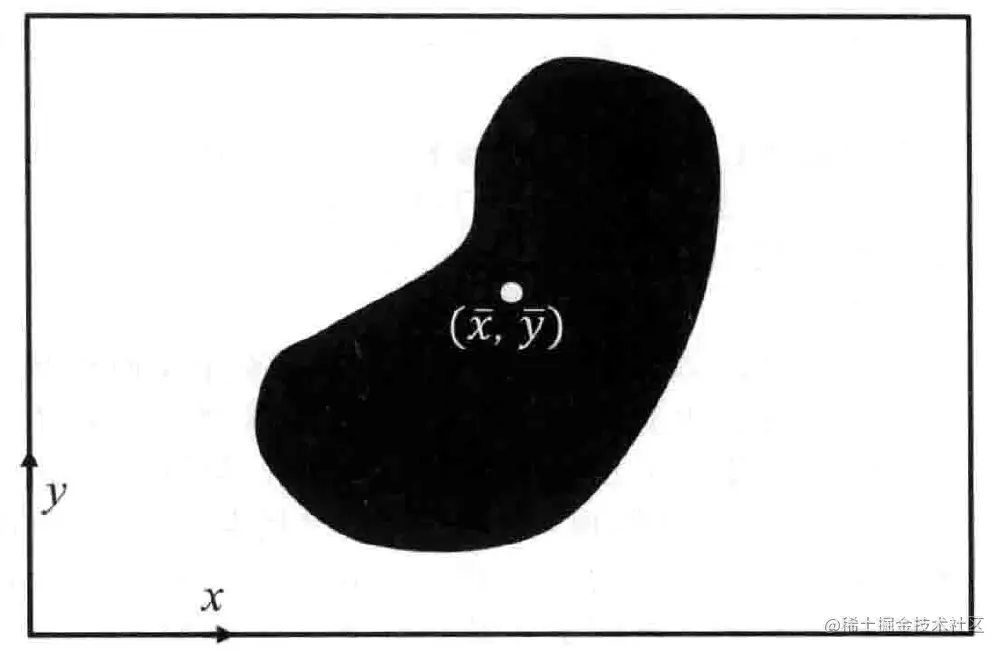
空间位置按照密度加权平均即是质心的位置 $(\bar{x}, \bar{y})$：

可以认为是二值图的 1 阶矩（静力矩）物理意义。

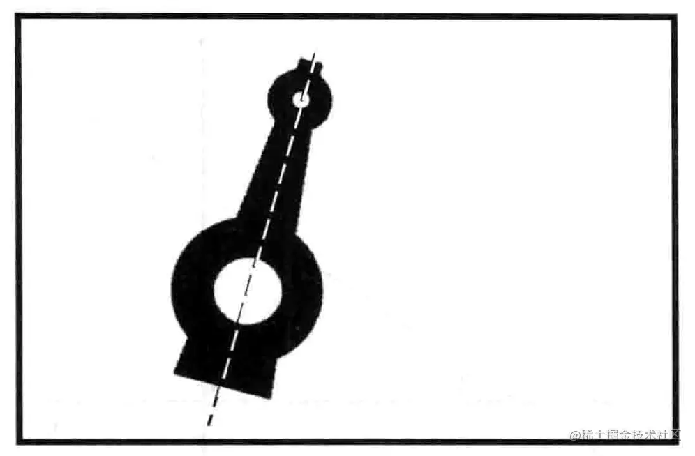
朝向

• 如果我们想要知道二值图物体表示的朝向，则需要用到转动惯量的概念。如果找到了使得物体转动惯量最小的轴，那么这个轴向就是物体的朝向。

• 在当前图像为二维的情况下，转动惯量是物体针对某条直线，将物体上的每个点到直线距离的平方按照密度计算积分，即得到了图像关于该轴向的转动惯量值。

• 我们的任务是为给定的二值图物体找到使得其转动惯量最小的直线。

• 转动惯量计算方法：

• 其中 $r$ 表示二值图上的点到直线的距离，虽然还没有这条直线

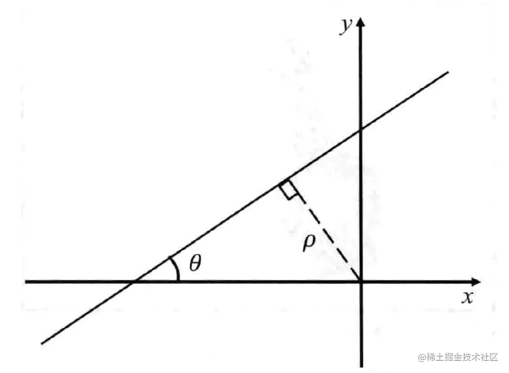
直线建模

• 为我们的目标直线建模，取2个参数

  • 原点到直线的距离 $\rho$
  • 直线和 $x$ 轴之间（沿逆时针方向）的夹角 $\theta$

• 这种建模方式有一些方便之处：

  • 当坐标系平移或旋转时，这两个参数的变化是连续的
  • 当直线平行（或近似平行）于某个坐标轴时，用这两个参数来表示直线也不会产生问题（相比于：使用斜率和截距来表示直线的情况）

• 使用这两个参数，可以将直线方程写为如下形式：

• 在直线上，距离原点最近的点$(-\rho \sin \theta,+\rho \cos \theta)$，通过这个点，沿着夹角 $\theta$ 运动任意距离$s$ 的点仍在直线上，因此可以将直线上任意一点$(x_0,y_0)$表示为：

最短距离

• 回到我们的二值图，在给定直线方程的情况下，二值图上一点$(x,y)$，直线上距离其最近的点$(x_0,y_0)$，二者距离显然可以表示为：

{%raw%}

{%endraw%}

• 将直线上点公式$\eqref{6}$代入，得到：

{%raw%}

{%endraw%}

• 对于每个点，我们都需要解$\eqref{8}$这样的优化方程
• 即给定了$x,y,\rho,\theta$，求解使得$r$最小的s,我们在$$\eqref{8}中对$s$求导，可得：

• 将$\eqref{9}$带入$\eqref{6}$，二值图上$(x,y)$到直线上距离最近的点$(x_0,y_0)$可得到关系为：

{%raw%}

{%endraw%}

• 将$\eqref{10}$带入 $\eqref{7}$可得：

• 此处可以看到，将某点$(x,y)$带入$\eqref{5}$，得到值的绝对值即为该点到直线的垂线（最短）距离。

二阶矩轴向通过质心

• 我们已经得到了二值图上一点到任意直线的距离计算方法，将$\eqref{11}$带入$\eqref{4}$，得到：

{%raw%}

{%endraw%}

• 对$\rho$求导，并令倒数为0，得到：

• 其中，A是区域面积，而是区域质心。因此，我们得到了结论：

确定轴向倾角

我们已经确定该轴经过一个确定的点$(\bar{x}, \bar{y})$了，仅需要再确定直线倾角即可。

• 将二值图平移到原点与质心重合的位置，那么我们要求得的就是一条穿过原点的直接倾角
• 也就是直接去除 $\rho$ 参数的影响
• 转动惯量计算方式如下：

其中，我们定义平移后的二值图$I'$上点的坐标为$({x'}, {y'})$。

• 可以表示为：

{%raw%}

{%endraw%}

• 即：

• 上式对$\theta$求导，并令求导结果等于零
• 假设$a≠c$，我们可以得到：

• 因此除非出现$b=0$ 并且 $a=c$ 的情况, 否则, 我们最终可以得到：

{%raw%}

{%endraw%}

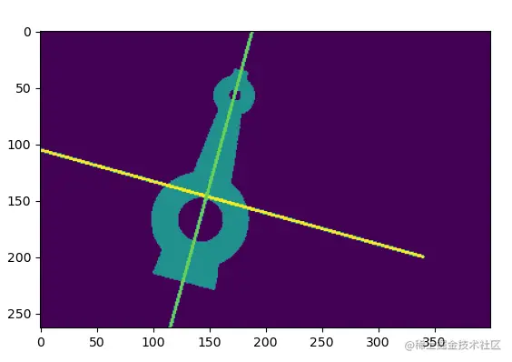
• 至此我们已经求出了使得该二值图转动惯量最小和最大的两个轴
• $E$​ 的的最小值和最大值的比值，给出了一些关于物体有“多么圆”的信息。对于直线，这个比值是0对于圆，这个比值是1。

拉格朗日

从式$\eqref{15}$开始，事实上我们要解的就是一个带约束的优化方程组，可以使用拉格朗日乘数法求解：

{%raw%}

{%endraw%}

• 将$E$设为$f(x,y)$，约束条件设为$g(x,y)=0$，构建拉格朗日方程：

• 构造拉格朗日方程组：

{%raw%}

{%endraw%}

• 重新令 $x = sin\theta, y=con\theta$可得：

{%raw%}

{%endraw%}

• 即推出$\eqref{17}$相同结论。

特征向量

可以将$\eqref{19}$看作是一个二次型优化问题，原带约束的方程可以写成：

{%raw%}

{%endraw%}

• 其中: {%raw%}${\bf{s}} = \left( \begin{array}{l} x\\ y \end{array} \right)${%endraw%}，{%raw%}{\bf{A}} = \left( \begin{array}{l} \begin{array}{*{20}{c}} a&{\frac{b}{2}} \end{array}\\ \begin{array}{*{20}{c}} {\frac{b}{2}}&c \end{array} \end{array} \right){%endraw%}，$\bf{I}$为二阶单位阵
• 那么拉格朗日方程可以写成：

{%raw%}

{%endraw%}

• $L$对$\bf{s}$的偏导数为0：

{%raw%}

{%endraw%}

• 而式$\eqref{25}$就是在寻找矩阵$\bf{A}$的特征向量和特征值。
• 也就是说，对于给定的二值图，求解其对应的$a,b,c$，构造出矩阵$\bf{A}$，求解$\bf{A}$的特征向量即是寻找最大、最小转动惯量的方向。
• 二者大小的比值也类似于特征值的比值，也就是矩阵的条件数。

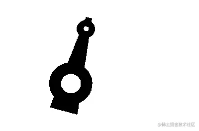
参考示例

• 示例图像：

• 示例程序

import math
import cv2

import numpy as np

import matplotlib.pyplot as plt
from numpy.lib.function_base import iterable


def vvd_round(num):
    if iterable(num):
        return np.round(np.array(num)).astype('int32').tolist()
    return int(round(num))


def show_image(image):
    plt.imshow(image.astype('uint8'))
    plt.show()
    pass


def gravity_center(mask):
    Ys, Xs = mask.nonzero()
    A = (mask > 0).sum()
    C_X = (Xs).sum() / A
    C_Y = (Ys).sum() / A
    return C_X, C_Y


def load_gray_image(image_path):
    image = cv2.imread(image_path)
    image = cv2.cvtColor(image, cv2.COLOR_BGR2GRAY)
    image = (image == 0).astype('uint8') * 255
    return image


def moment_of_inertia(mask, center):
    temp_image = mask.copy().astype('uint8') * 128

    C_X, C_Y = center

    Ys, Xs = mask.nonzero()

    Ys = (Ys - C_Y) / 100
    Xs = (Xs - C_X) / 100

    a = (Xs * Xs).sum()
    b = 2 * (Xs * Ys).sum()
    c = (Ys * Ys).sum()

    if b == 0:
        theta = 0
    elif a == c:
        theta = - np.pi * 0.5 * 0.5
    else:
        theta = - math.atan(b / (a - c)) / 2

    point_1 = vvd_round([C_X + math.cos(theta) * 200, C_Y - math.sin(theta) * 200])
    point_2 = vvd_round([C_X - math.cos(theta) * 200, C_Y + math.sin(theta) * 200])

    temp_image = cv2.line(temp_image.astype('uint8'), point_1, point_2, 255, 2)

    point_1 = vvd_round([C_X + math.cos(theta + 0.5 * np.pi) * 200, C_Y - math.sin(theta + 0.5 * np.pi) * 200])
    point_2 = vvd_round([C_X - math.cos(theta + 0.5 * np.pi) * 200, C_Y + math.sin(theta + 0.5 * np.pi) * 200])

    temp_image = cv2.line(temp_image.astype('uint8'), point_1, point_2, 200, 2)

    theta_1 = theta
    theta_2 = theta + 0.5 * np.pi

    E_1 =(math.sin(theta_1)) ** 2 * a - b * math.sin(theta_1) * math.cos(theta_1) + c * (math.cos(theta_1)) ** 2
    E_2 =(math.sin(theta_2)) ** 2 * a - b * math.sin(theta_2) * math.cos(theta_2) + c * (math.cos(theta_2)) ** 2

    return temp_image, min(E_2, E_1) / max(E_2, E_1, 1)


if __name__ == '__main__':
    image_path = 'test.png'
    image = load_gray_image(image_path)
    center = gravity_center(image)
    temp_image, rate = moment_of_inertia(image, center)
    show_image(temp_image)
    pass

• 示例效果

参考资料

• 伯特霍尔德・霍恩著BERTHOLDKLAUSPAULHORN. 机器视觉[M]. 中国青年出版社, 2014.