

AutoML搜索HPO简单实战
本文简单的介绍如何使用ray中的tune的功能来搜索网络超参数。一个模型的成功其实离不开精心挑选设定的超参数,而超参数本身与模型的训练过程,硬件条件其实是密切相关的。很多算法在Paper只会给你展示最终的结果,而过程中经历的无数失败的参数尝试却根本不会体现出来。 很多人调侃AutoML抢了ai工程师的饭碗,其实ai工程师作的事情并不只是调参(质疑)。能够写出这样的自动化的工具,其把自己的模型最佳搭配参数找出来,那也是只有ai工程师能做的事情。本文就来教大家来如何入门。
这里使用的工具只有一个,那就是ray,关于ray的介绍大家可以看官网,你可以把他看作是ai界的scalar,在某些时候这种工具还是挺管用的,我们不需要用到他的所有功能,这里只需要用到他的一个模块,tune。
pip install ray
pip install alfred-py
ray做超参搜索
其实用ray来做HPO非常简单,我们以一个分类任务为例子,这里的模型是我们自己定义的,一个非常简单的ConvNet,然后我们采用sgd进行优化,我们希望知道在我们的target 硬件,也就是一个GPU下,最佳的lr以及momentum是多少,请注意,这里不是无脑的0.1和0.9,这些都是经验值,经验值一定最优吗?还真不一定,这也是为什么你需要做这么一步的原因。
废话不多说,直接上代码:
'''
this projects demonstrate how to tune
hyper parameters on a model
'''
from ray.tune.schedulers import ASHAScheduler
import numpy as np
import torch
import torch.optim as optim
import torch.nn as nn
import torch.nn.functional as F

from ray import tune
from ray.tune.examples.mnist_pytorch import get_data_loaders, train, test
import ray
import sys
from alfred.dl.torch.common import device


if len(sys.argv) > 1:
    ray.init(redis_address=sys.argv[1])


class ConvNet(nn.Module):
    def __init__(self):
        super(ConvNet, self).__init__()
        self.conv1 = nn.Conv2d(1, 3, kernel_size=3)
        self.fc = nn.Linear(192, 10)

    def forward(self, x):
        x = F.relu(F.max_pool2d(self.conv1(x), 3))
        x = x.view(-1, 192)
        x = self.fc(x)
        return F.log_softmax(x, dim=1)


def train_mnist(config):
    model = ConvNet()
    model.to(device)
    train_loader, test_loader = get_data_loaders()
    optimizer = optim.SGD(
        model.parameters(), lr=config["lr"], momentum=config["momentum"])
    for i in range(10):
        train(model, optimizer, train_loader, device)
        acc = test(model, test_loader, device)
        # tune.track.log(mean_accuracy=acc)
        tune.report(mean_accuracy=acc)
        if i % 5 == 0:
            # This saves the model to the trial directory
            torch.save(model.state_dict(), "./model.pth")


search_space = {
    "lr": tune.choice([0.001, 0.01, 0.1]),
    "momentum": tune.uniform(0.1, 0.9)
}

analysis = tune.run(
    train_mnist,
    num_samples=30,
    resources_per_trial={'gpu': 1},
    scheduler=ASHAScheduler(metric="mean_accuracy",
                            mode="max", grace_period=1),
    config=search_space)
真的是超级简单,就这么即行代码,你可以对你的超参数进行优化了。运行完成之后,你可以看到类似于这样的输出:
Number of trials: 30/30 (30 TERMINATED)
+-------------------------+------------+-------------------+-------+------------+----------+--------+------------------+
| Trial name              | status     | loc               |    lr |   momentum |      acc |   iter |   total time (s) |
|-------------------------+------------+-------------------+-------+------------+----------+--------+------------------|
| train_mnist_f71cb_00000 | TERMINATED | 10.80.43.74:55628 | 0.001 |   0.338473 | 0.1      |     10 |          3.4553  |
| train_mnist_f71cb_00001 | TERMINATED | 10.80.43.74:55629 | 0.001 |   0.333578 | 0.2375   |     10 |          3.35463 |
| train_mnist_f71cb_00002 | TERMINATED | 10.80.43.74:55632 | 0.1   |   0.765898 | 0.865625 |     10 |          3.3302  |
| train_mnist_f71cb_00003 | TERMINATED | 10.80.43.74:55627 | 0.01  |   0.109677 | 0.290625 |      1 |          2.19001 |
| train_mnist_f71cb_00004 | TERMINATED | 10.80.43.74:55633 | 0.01  |   0.25874  | 0.24375  |      1 |          2.23142 |
| train_mnist_f71cb_00005 | TERMINATED | 10.80.43.74:55630 | 0.01  |   0.586889 | 0.2125   |      1 |          2.24251 |
| train_mnist_f71cb_00006 | TERMINATED | 10.80.43.74:55631 | 0.001 |   0.159626 | 0.128125 |      1 |          2.22076 |
| train_mnist_f71cb_00007 | TERMINATED | 10.80.43.74:55622 | 0.01  |   0.880302 | 0.890625 |     10 |          3.35615 |
| train_mnist_f71cb_00008 | TERMINATED | 10.80.43.74:55620 | 0.001 |   0.824616 | 0.0625   |      1 |          2.24873 |
| train_mnist_f71cb_00009 | TERMINATED | 10.80.43.74:55618 | 0.001 |   0.520118 | 0.025    |      1 |          2.21357 |
| train_mnist_f71cb_00010 | TERMINATED | 10.80.43.74:55621 | 0.001 |   0.374901 | 0.1625   |      1 |          2.21661 |
| train_mnist_f71cb_00011 | TERMINATED | 10.80.43.74:55626 | 0.1   |   0.380379 | 0.840625 |     10 |          3.29623 |
| train_mnist_f71cb_00012 | TERMINATED | 10.80.43.74:55619 | 0.001 |   0.16643  | 0.103125 |      1 |          2.18452 |
| train_mnist_f71cb_00013 | TERMINATED | 10.80.43.74:55624 | 0.01  |   0.83129  | 0.753125 |      4 |          2.62007 |
| train_mnist_f71cb_00014 | TERMINATED | 10.80.43.74:55625 | 0.1   |   0.302737 | 0.76875  |      4 |          2.55607 |
| train_mnist_f71cb_00015 | TERMINATED | 10.80.43.74:55623 | 0.001 |   0.10079  | 0.14375  |      1 |          2.19084 |
| train_mnist_f71cb_00016 | TERMINATED | 10.80.43.74:56210 | 0.01  |   0.310645 | 0.221875 |      1 |          2.15354 |
| train_mnist_f71cb_00017 | TERMINATED | 10.80.43.74:56244 | 0.1   |   0.302933 | 0.8625   |     10 |          3.40914 |
| train_mnist_f71cb_00018 | TERMINATED | 10.80.43.74:56288 | 0.1   |   0.472268 | 0.88125  |     10 |          3.36956 |
| train_mnist_f71cb_00019 | TERMINATED | 10.80.43.74:56344 | 0.01  |   0.368897 | 0.0875   |      1 |          2.17568 |
| train_mnist_f71cb_00020 | TERMINATED | 10.80.43.74:56376 | 0.1   |   0.87095  | 0.959375 |     10 |          3.41518 |
| train_mnist_f71cb_00021 | TERMINATED | 10.80.43.74:56410 | 0.1   |   0.225298 | 0.834375 |      4 |          2.65473 |
| train_mnist_f71cb_00022 | TERMINATED | 10.80.43.74:56447 | 0.001 |   0.385364 | 0.15625  |      1 |          2.2179  |
| train_mnist_f71cb_00023 | TERMINATED | 10.80.43.74:56480 | 0.1   |   0.455948 | 0.846875 |      4 |          2.60914 |
| train_mnist_f71cb_00024 | TERMINATED | 10.80.43.74:56531 | 0.001 |   0.643994 | 0.103125 |      1 |          2.20683 |
| train_mnist_f71cb_00025 | TERMINATED | 10.80.43.74:56565 | 0.01  |   0.525646 | 0.246875 |      1 |          2.19718 |
| train_mnist_f71cb_00026 | TERMINATED | 10.80.43.74:56602 | 0.1   |   0.178208 | 0.7      |      4 |          2.60433 |
| train_mnist_f71cb_00027 | TERMINATED | 10.80.43.74:56635 | 0.001 |   0.557703 | 0.11875  |      1 |          2.27553 |
| train_mnist_f71cb_00028 | TERMINATED | 10.80.43.74:56667 | 0.001 |   0.360534 | 0.046875 |      1 |          2.30704 |
| train_mnist_f71cb_00029 | TERMINATED | 10.80.43.74:56713 | 0.001 |   0.466288 | 0.13125  |      1 |          2.31522 |
+-------------------------+------------+-------------------+-------+------------+----------+--------+------------------+


2022-02-08 16:08:57,847	INFO tune.py:636 -- Total run time: 172.06 seconds (171.83 seconds for the tuning loop).
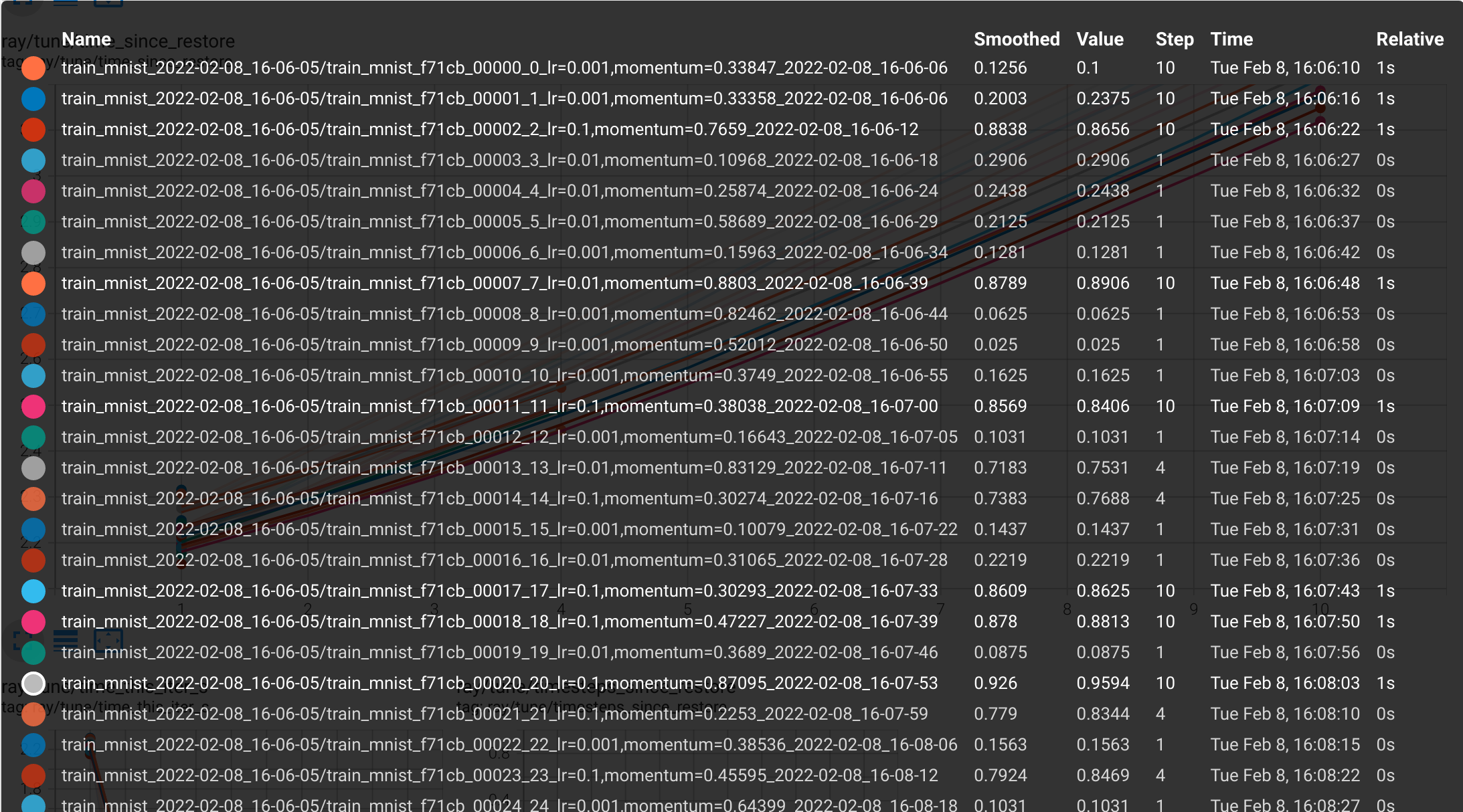
如果你安装了tensorboard,你还可以看到类似于这样的曲线:
一眼就能看出,高亮的地方就是你的最优化的参数:
这个效果还算不错。直接可以找到一个最合适的超参数配置,搭配你的模型,一定可以实现无疑伦比的精度。
Ray是否可以扩展到大型检测网络超参数搜索
答案当然是可以的,只是比较麻烦。在我之前开源的YOLOv7系列中,就有很多模型的组合,每个模型的组合其实对超参数依赖都不同。这里贴一段给大家参考的可以对大型训练框架,进行超参数搜索的案例:
import detectron2
from detectron2.utils.logger import setup_logger
setup_logger()

import detectron2.data.transforms as T

# import some common detectron2 utilities
from detectron2 import model_zoo
from detectron2.data import detection_utils as utils
from detectron2.data import MetadataCatalog, DatasetCatalog, build_detection_train_loader, DatasetMapper, build_detection_test_loader
from detectron2.engine import DefaultTrainer, DefaultPredictor
from detectron2.config import get_cfg
from detectron2.evaluation import COCOEvaluator, inference_on_dataset
from detectron2.engine.hooks import HookBase
from detectron2.data.datasets import register_coco_instances, load_coco_json
from detectron2.utils.visualizer import Visualizer, ColorMode
from detectron2.structures.boxes import BoxMode

import numpy as np
import os, json, cv2, random

# import PointRend project
from detectron2.projects import point_rend

import copy
import torch
import matplotlib.pyplot as plt
from PIL import Image, ImageDraw

from torchvision.transforms import functional as F
import random
import albumentations as A

# Hyperparametertuning
import ray
from functools import partial
from ray import tune
from ray.tune import JupyterNotebookReporter
from ray.tune.schedulers import ASHAScheduler

# %% [markdown]
# # Register the train and test dataset

# %% [code]
def get_balloon_dicts(img_dir):
    json_file = os.path.join(img_dir, "via_region_data.json")
    with open(json_file) as f:
        imgs_anns = json.load(f)

    dataset_dicts = []
    for idx, v in enumerate(imgs_anns.values()):
        record = {}

        filename = os.path.join(img_dir, v["filename"])
        height, width = cv2.imread(filename).shape[:2]

        record["file_name"] = filename
        record["image_id"] = idx
        record["height"] = height
        record["width"] = width

        annos = v["regions"]
        objs = []
        for _, anno in annos.items():
            assert not anno["region_attributes"]
            anno = anno["shape_attributes"]
            px = anno["all_points_x"]
            py = anno["all_points_y"]
            poly = [(x + 0.5, y + 0.5) for x, y in zip(px, py)]
            poly = [p for x in poly for p in x]

            obj = {
                "bbox": [np.min(px), np.min(py), np.max(px), np.max(py)],
                "bbox_mode": BoxMode.XYXY_ABS,
                "segmentation": [poly],
                "category_id": 0,
                'iscrowd': 0,
            }
            objs.append(obj)
        record["annotations"] = objs
        dataset_dicts.append(record)
    return dataset_dicts

for d in ["train", "val"]:
    DatasetCatalog.register("balloon_" + d, lambda d=d: get_balloon_dicts("balloon/" + d))
    MetadataCatalog.get("balloon_" + d).set(thing_classes=["balloon"])
balloon_metadata = MetadataCatalog.get("balloon_train")

# %% [markdown]
# # Generate the custom Trainer class using augmentations and hook

# %% [code]
class RayTuneReporterHook(HookBase):
    """ SEMI IMPLEMENTED: Hook for Ray Tune Reporter"""
    def __init__(self, eval_period):
        self._eval_period = eval_period

    def after_step(self):
        next_iter = self.trainer.iter + 1
        is_final = next_iter == self.trainer.max_iter
        if is_final or (self._eval_period > 0 and next_iter % self._eval_period == 0):
            loss_mask_latest = self.trainer.storage.history('loss_mask').latest()
            tune.report(loss_mask=loss_mask_latest)
            print(f'{self.trainer.iter}: losses and mAPs {loss_mask_latest}')

class CustomTrainer(DefaultTrainer):
    """ Custom trainer class"""

    def __init__(self, cfg, hp):
        self._hp = hp
        super().__init__(cfg)

    def build_hooks(self):
        # build hooks from super class
        # and add ray tune reporter hook
        hooks = super().build_hooks()
        hooks.insert(-1,RayTuneReporterHook(self.cfg.TEST.EVAL_PERIOD))
        return hooks

# %% [markdown]
# # Train the PointRend model

# %% [code]
def set_cfg_values(hp):
    """ Set the Config values for the PointRend model"""
    cfg = get_cfg()
    # Add PointRend-specific config
    point_rend.add_pointrend_config(cfg)
    # Load a config from file
    cfg.merge_from_file("/kaggle/working/detectron2_repo/projects/PointRend/configs/InstanceSegmentation/pointrend_rcnn_R_50_FPN_3x_coco.yaml")
    cfg.MODEL.ROI_HEADS.SCORE_THRESH_TEST = 0.5  # set threshold for this model
    cfg.DATASETS.TRAIN = ("balloon_train",)
    cfg.DATASETS.TEST = ("balloon_val",)
    cfg.DATALOADER.NUM_WORKERS = 4
    # Use a model from PointRend model zoo: https://github.com/facebookresearch/detectron2/tree/master/projects/PointRend#pretrained-models
    cfg.MODEL.WEIGHTS = "detectron2://PointRend/InstanceSegmentation/pointrend_rcnn_R_50_FPN_3x_coco/164955410/model_final_edd263.pkl"
    cfg.MODEL.ROI_HEADS.BATCH_SIZE_PER_IMAGE = 512 #128   # faster, and good enough for this toy dataset (default: 512)
    cfg.MODEL.ROI_HEADS.NUM_CLASSES = 1  # only has one class (ballon). (see https://detectron2.readthedocs.io/tutorials/datasets.html#update-the-config-for-new-datasets)
    cfg.MODEL.POINT_HEAD.NUM_CLASSES = 1  # only has one class (ballon). (see https://detectron2.readthedocs.io/tutorials/datasets.html#update-the-config-for-new-datasets)
    # NOTE: this config means the number of classes, but a few popular unofficial tutorials incorrect uses num_classes+1 here.
    cfg.SEED = 1
    cfg.INPUT.FORMAT = 'RGB'
    cfg.INPUT.RANDOM_FLIP = 'none'
    cfg.TEST.EVAL_PERIOD = 1

    # Hyperparams that need to be solved
    cfg.OUTPUT_DIR = '/kaggle/working/output'
    cfg.SOLVER.IMS_PER_BATCH = hp['batch_size']
    cfg.SOLVER.BASE_LR = hp['lr'] #0.00025  # pick a good LR
    cfg.SOLVER.MAX_ITER = hp['epochs'] #300    # 300 iterations seems good enough for this toy dataset; you will need to train longer for a practical dataset
    cfg.SOLVER.STEPS = (3,) #[]        # do not decay learning rate

    if hp['anchorboxes']:
        cfg.MODEL.ANCHOR_GENERATOR.SIZES = [[8, 16, 32, 64, 128]]
        cfg.MODEL.ANCHOR_GENERATOR.ASPECT_RATIOS = [[0.25, 0.5, 1.0, 2.0]]
    return cfg

# %% [code]
def train_model(hp, checkpoint_dir=None):
    cfg = set_cfg_values(hp)
    # Train the model
    os.makedirs(cfg.OUTPUT_DIR, exist_ok=True)
    trainer = CustomTrainer(cfg, hp)
    trainer.resume_or_load(resume=False)
    trainer.train()

# %% [code]
# This plain cell works
hp = {"epochs": 8,
              "lr": 1e-3,
              "batch_size": 2,
              "anchorboxes": False,
              "hflip": 0.5,
              "vflip": 0.5,
              "blur": 0.5,
              "contrast": 0.2,
              "brightness": 0.2}
train_model(hp)

# %% [code]
# And this hyperparameter function cell does not
def main(num_samples=10, max_num_epochs=10, gpus_per_trial=1):
    # Set the hyperparameter configuration dict with viable ranges
    hp = {"epochs": tune.randint(8,15),
              "lr": tune.loguniform(1e-3, 1e-2),
              "batch_size": tune.choice([2, 4, 8]),
              "anchorboxes": False,
              "hflip": tune.choice([0, 0.5]),
              "vflip": tune.choice([0, 0.5]),
              "blur": tune.choice([0, 0.5]),
              "contrast": tune.choice([0, 0.2]),
              "brightness": tune.choice([0, 0.2])}

    # initialize tha Asynchronous Successive Halving Algorithm Scheduler
    scheduler = ASHAScheduler(
        metric="loss_mask",
        mode="min",
        max_t=max_num_epochs,
        grace_period=1,
        reduction_factor=4)

    # Report results to the CLI
    reporter = JupyterNotebookReporter(overwrite=False,
                                       metric_columns=["loss_mask", "segm_map_small",
                                                       "segm_map_medium", "training_iteration"])

    # Run the ASHA algorithm
    result = tune.run(
        train_model,
        resources_per_trial={"cpu": 2, "gpu": gpus_per_trial},
        config=hp,
        num_samples=num_samples,
        scheduler=scheduler,
        progress_reporter=reporter)

    # Get the best model
    best_trial = result.get_best_trial("loss_mask", "min", "last")
    print("Best trial config: {}".format(best_trial.config))
    print("Best trial final validation loss: {}".format(
        best_trial.last_result["loss_mask"]))
    print("Best trial final validation segm_map_small: {}".format(
        best_trial.last_result["segm_map_small"]))
    print("Best trial final validation segm_map_medium: {}".format(
        best_trial.last_result["segm_map_medium"]))

if __name__ == "__main__":
    # You can change the number of GPUs per trial here:
    main(num_samples=2, max_num_epochs=3, gpus_per_trial=1)
总结
ray是一个不错的工具,做分布式计算和搜索大有用途,感兴趣的童鞋可以好好研究研究。
打个小广告: github.com/jinfagang/y…
