math作业中关于梯度下降算法的一个实现过程
from matplotlib import pyplot as plt
from mpl_toolkits.mplot3d import Axes3D
import numpy as np
from matplotlib import cm
from numpy import random
d额
# Definition of draw surface of F0 or F1
def DrawSurface(fig, varxrange, varyrange, function, ax):
xx, yy = np.meshgrid(varxrange, varyrange, sparse=False) # 1D to 2D
z = function(xx, yy)
ax.plot_wireframe(xx, yy, z)
fig.canvas.draw()
# Definition of F0
def F0(x, y):
return 1.5 - 1.6 * np.exp(-0.05 * (3 * (x + 3) ** 2 + (y + 3) ** 2))
# Definition of gradient of F0
def F0Grad(x, y):
g = np.zeros(2)
g[0] = -1.6 * (-0.3 * x - 0.9) * np.exp(-0.15 * (x + 3) ** 2 - 0.05 * (y + 3) ** 2)
g[1] = -1.6 * (-0.1 * y - 0.3) * np.exp(-0.15 * (x + 3) ** 2 - 0.05 * (y + 3) ** 2)
return g
# Definition of F1
def F1(x, y):
F = 1.5 - 1.6 * np.exp(-0.05 * (3 * (x + 3) ** 2 + (y + 3) ** 2))
return F + (0.5 - np.exp(-0.1 * (3 * (x - 3) ** 2 + (y - 3) ** 2)))
# Definition of gradient of F1
def F1Grad(x, y):
g = np.zeros(2)
g[0] = -(1.8 - 0.6 * x) * np.exp(-0.3 * (x - 3) ** 2 - 0.1 * (y - 3) ** 2) - 1.6 * (-0.3 * x - 0.9) * np.exp(
-0.15 * (x + 3) ** 2 - 0.05 * (y + 3) ** 2)
g[1] = -(0.6 - 0.2 * y) * np.exp(-0.3 * (x - 3) ** 2 - 0.1 * (y - 3) ** 2) - 1.6 * (-0.1 * y - 0.3) * np.exp(
-0.15 * (x + 3) ** 2 - 0.05 * (y + 3) ** 2)
return g
# Function implementing gradient descent of F0
def GradDescent0(StartPt, LRate, i, xx, yy, zz):
global m0
while 1:
# TO DO: Calculate the 'height' at StartPt using F0 or F1
i = i+1
if i == 10000000:
i = random.randint(10000000, 44444444)
print(str(i) + " times")
m0 += float(i) / 625
return 1
x, y = StartPt
z0 = F0(x, y)
GetPoint0(x, y, z0, xx, yy, zz)
# TO DO: Calculate the gradient at StartPt
g0 = F0Grad(x, y)
# TO DO: Calculate the new point and update StartPoint
x = x - g0[0] * LRate
y = y - g0[1] * LRate
if abs(z0 - F0(x, y)) < 1e-65:
print(str(i) + " times")
m0 += float(i)/2500
if z0 < 0.09999999:
return 1
return 0
StartPt = np.array([x, y])
# Make sure StartPt is within the specified bounds
StartPt = np.maximum(StartPt, [-7, -7])
StartPt = np.minimum(StartPt, [7, 7])
# Function implementing gradient descent of F1
def GradDescent1(StartPt, LRate, i, xx, yy, zz):
global m1
while 1:
# TO DO: Calculate the 'height' at StartPt using F0 or F1
i = i + 1
if i == 10000000:
i = random.randint(10000000, 44444444)
print(str(i) + " times")
m1 += float(i) / 625
return 1
x, y = StartPt
z1 = F1(x, y)
GetPoint1(x, y, z1, xx, yy, zz)
# TO DO: Calculate the gradient at StartPt
g1 = F1Grad(x, y)
# TO DO: Calculate the new point and update StartPoint
x = x - g1[0] * LRate
y = y - g1[1] * LRate
if abs(z1 - F1(x, y)) < 1e-65:
print(str(i) + " times")
m1 += float(i)/2500
if z1 < 0.4:
return 1
return 0
StartPt = np.array([x, y])
# Make sure StartPt is within the specified bounds
StartPt = np.maximum(StartPt, [-7, -7])
StartPt = np.minimum(StartPt, [7, 7])
# Record the coordinates of the points passed during the execution of the gradient descent algorithm of F0
def GetPoint0(x, y, z, xx, yy, zz):
xx.append(x)
yy.append(y)
zz.append(z)
# Record the coordinates of the points passed during the execution of the gradient descent algorithm of F1
def GetPoint1(x, y, z, xx, yy, zz):
xx.append(x)
yy.append(y)
zz.append(z)
# Used to filter the array value that can reach the optimal solution in the point set in F0
def JudgePt0(LRate, v, xx, yy, zz):
global num0
t = 20
z = [[0 for i in range(0, t)]for j in range(0, t)]
x = np.linspace(-7, 7, t)
y = np.linspace(-7, 7, t)
X, Y = np.meshgrid(x, y)
for i in range(t):
for j in range(t):
z[i][j] = GradDescent0([x[i], y[j]], LRate, v, xx, yy, zz)
if z[i][j]:
num0 += 1
Z = np.array(z)
Z.reshape(t, t)
return X, Y, Z
# Used to filter the array value that can reach the optimal solution in the point set in F1
def JudgePt1(LRate, v, xx, yy, zz):
global num1
t = 20
z = [[0 for i in range(0, t)]for j in range(0, t)]
x = np.linspace(-7, 7, t)
y = np.linspace(-7, 7, t)
X, Y = np.meshgrid(x, y)
for i in range(t):
for j in range(t):
z[i][j] = GradDescent1([x[i], y[j]], LRate, v, xx, yy, zz)
if z[i][j]:
num1 += 1
Z = np.array(z)
Z.reshape(t, t)
return X, Y, Z
m0 = 0. # Mean of iterations in F0
m1 = 0. # Mean of iterations in F1
num0 = 0 # The number of points which can arrive the minimum in F0.
num1 = 0 # The number of points which can arrive the minimum in F1.
def main():
# Define initial variables
x0 =[]
y0 =[]
z0 =[]
x1 =[]
y1 =[]
z1 =[] # These lists are used to store the collection of points
LRate = 0.01 # Learn rate
i = 0 # Used to record the number of iterations
# TO DO: choose a random starting point with x and y in the range (-7, 7)
# random.seed(0)
x = random.uniform(-7, 7)
y = random.uniform(-7, 7)
StartPt = np.array([x, y]) # to array
print("The random points is :")
print(StartPt)
# Find minimum
v1 = GradDescent0(StartPt, LRate, i, x0, y0, z0)
if v1:
print("The pt can arrive the minimum in F0")
else:
print("The pt can not arrive the minimum in F0")
v2 = GradDescent1(StartPt, LRate, i, x1, y1, z1)
if v2:
print("The pt can arrive the minimum in F1")
else:
print("The pt can not arrive the minimum in F1")
# Drawing
fig = plt.figure(figsize=(18, 9), facecolor='w')
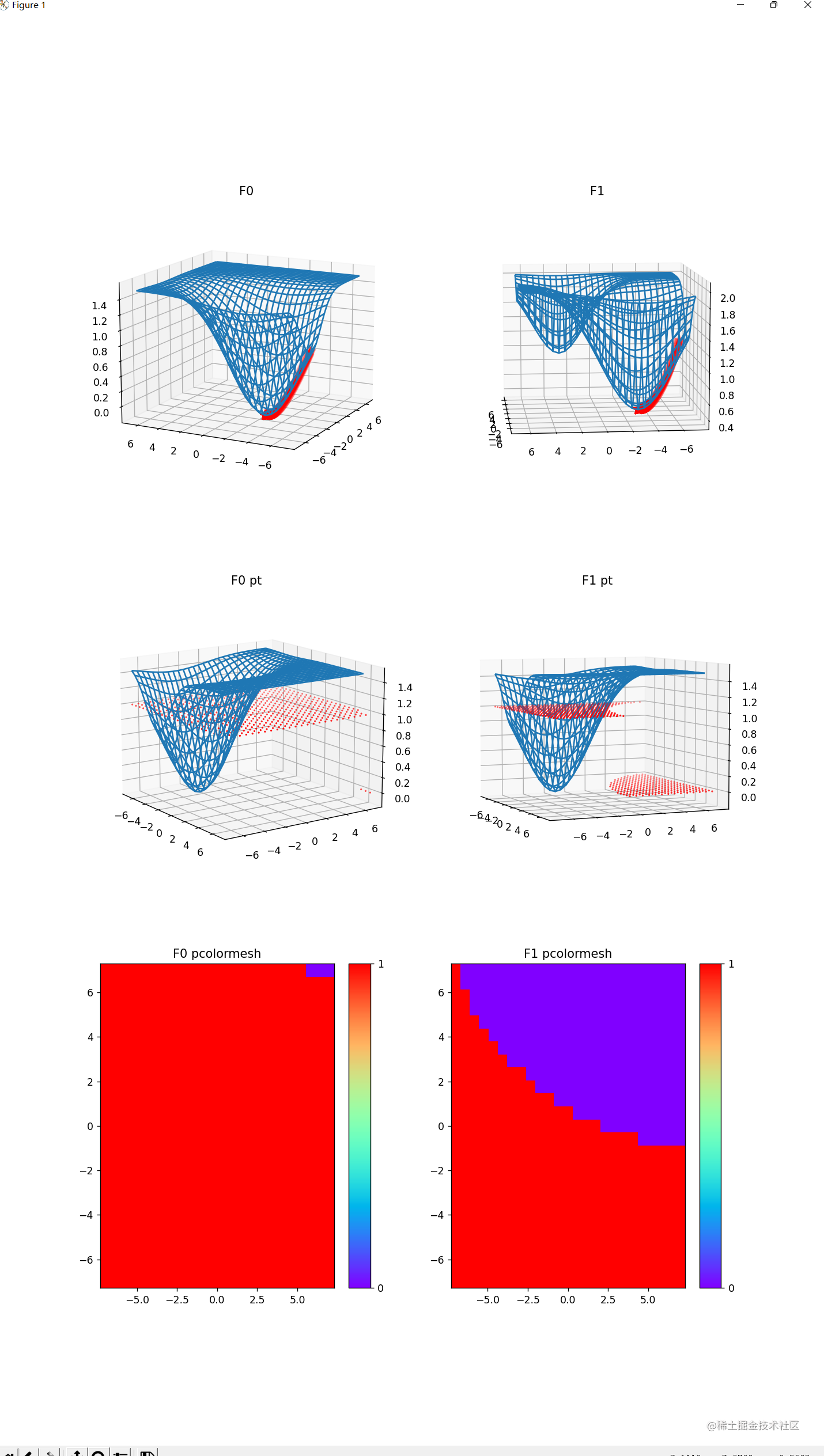
# 1.The gradient descent process of F0
ax = fig.add_subplot(321, projection='3d')
ax.scatter(x0, y0, z0, alpha=0.3, c="#FF0000", s=100, depthshade=True, marker='*')
DrawSurface(fig, np.arange(-7, 7, 0.5), np.arange(-7, 7, 0.5), F0, ax)
plt.title(u'F0')
plt.grid(True)
# 2.The gradient descent process of F1
ax2 = fig.add_subplot(322, projection='3d')
ax2.scatter(x1, y1, z1, alpha=0.3, c="#FF0000", s=100, depthshade=True, marker='*')
DrawSurface(fig, np.arange(-7, 7, 0.5), np.arange(-7, 7, 0.5), F1, ax2)
plt.title(u'F1')
plt.grid(True)
# 3.Mark which points can reach the minimum value in the 3D diagram, and use 0 or 1 to distinguish in F0
X0, Y0, Z0 = JudgePt0(LRate, i, x0, y0, z0)
ax3 = fig.add_subplot(323, projection='3d')
ax3.scatter(X0, Y0, Z0, s=1, c='r', depthshade=True, marker='*')
DrawSurface(fig, np.arange(-7, 7, 0.5), np.arange(-7, 7, 0.5), F0, ax3)
plt.title(u'F0 pt')
plt.grid(True)
# 4.Mark which points can reach the minimum value in the 3D diagram, and use 0 or 1 to distinguish in F1
X1, Y1, Z1 = JudgePt1(LRate, i, x1, y1, z1)
ax4 = fig.add_subplot(324, projection='3d')
ax4.scatter(X1, Y1, Z1, s=1, c='r', depthshade=True, marker='*')
DrawSurface(fig, np.arange(-7, 7, 0.5), np.arange(-7, 7, 0.5), F0, ax4)
plt.title(u'F1 pt')
plt.grid(True)
# 5.Test the algorithm for F0 systematically by using the function pcolormesh.
sub = fig.add_subplot(325)
pm = sub.pcolormesh(X0, Y0, Z0, cmap='rainbow')
fig.colorbar(pm, aspect=15, shrink=1, ticks=[1, 0])
plt.title(u'F0 pcolormesh')
# 6.Test the algorithm for F1 systematically by by using the function pcolormesh.
sub2 = fig.add_subplot(326)
pm2 = sub2.pcolormesh(X1, Y1, Z1, cmap='rainbow')
fig.colorbar(pm2, aspect=15, shrink=1, ticks=[1, 0])
plt.title(u'F1 pcolormesh')
# Output means of steps
print("Mean of iterations in F0 is : " + str(m0))
print("Mean of iterations in F1 is : " + str(m1))
print("The number of points which can arrive the minimum in F0 is : " + str(num0))
print("The number of points which can arrive the minimum in F0 is : " + str(num1))
plt.show()
if __name__ == "__main__":
main()
"""
F0
-2.9999999999999956 -2.999999372960323 -0.09999999999996767
F1
-2.999995819486321 -2.999995163550212 0.3999994426040736
"""
最终效果