TensorFlow 从入门到精通（1）—— 单变量线性回归

SGD

import tensorflow as tf
import numpy as np
import matplotlib.pyplot as plt 

tf.__version__

'2.5.1'

一、准备数据集

x = np.linspace(-2,2,100)
x

array([-2.        , -1.95959596, -1.91919192, -1.87878788, -1.83838384,
       -1.7979798 , -1.75757576, -1.71717172, -1.67676768, -1.63636364,
       -1.5959596 , -1.55555556, -1.51515152, -1.47474747, -1.43434343,
       -1.39393939, -1.35353535, -1.31313131, -1.27272727, -1.23232323,
       -1.19191919, -1.15151515, -1.11111111, -1.07070707, -1.03030303,
       -0.98989899, -0.94949495, -0.90909091, -0.86868687, -0.82828283,
       -0.78787879, -0.74747475, -0.70707071, -0.66666667, -0.62626263,
       -0.58585859, -0.54545455, -0.50505051, -0.46464646, -0.42424242,
       -0.38383838, -0.34343434, -0.3030303 , -0.26262626, -0.22222222,
       -0.18181818, -0.14141414, -0.1010101 , -0.06060606, -0.02020202,
        0.02020202,  0.06060606,  0.1010101 ,  0.14141414,  0.18181818,
        0.22222222,  0.26262626,  0.3030303 ,  0.34343434,  0.38383838,
        0.42424242,  0.46464646,  0.50505051,  0.54545455,  0.58585859,
        0.62626263,  0.66666667,  0.70707071,  0.74747475,  0.78787879,
        0.82828283,  0.86868687,  0.90909091,  0.94949495,  0.98989899,
        1.03030303,  1.07070707,  1.11111111,  1.15151515,  1.19191919,
        1.23232323,  1.27272727,  1.31313131,  1.35353535,  1.39393939,
        1.43434343,  1.47474747,  1.51515152,  1.55555556,  1.5959596 ,
        1.63636364,  1.67676768,  1.71717172,  1.75757576,  1.7979798 ,
        1.83838384,  1.87878788,  1.91919192,  1.95959596,  2.        ])

y = 3 * x + 1 + np.random.randn(*x.shape)*0.4
y

array([-4.6270979 , -4.53208454, -5.09927372, -4.31308491, -4.89209532,
       -3.83879435, -4.2554199 , -4.79988   , -3.5295878 , -3.34996221,
       -3.50203211, -3.4493262 , -3.67082173, -3.53057077, -3.37949467,
       -3.39710176, -2.76097088, -2.98001098, -3.38182339, -2.51148793,
       -2.62293237, -2.55154768, -2.18731766, -2.74440457, -1.68705141,
       -2.85560784, -1.72040223, -1.79404523, -1.14630636, -1.39208413,
       -1.52531324, -1.26251851, -1.25248595, -0.99099478, -1.15877518,
       -0.97176174, -0.699788  , -0.72376198, -0.06971146, -0.34889405,
       -0.58573642, -0.40268934, -0.3564667 ,  0.05316242,  0.8782646 ,
       -0.17009761,  0.36786618,  0.76453272,  1.50452912,  1.26186933,
        1.36393192,  1.4067708 ,  1.66703971,  0.58272023,  1.18168293,
        1.36694984,  2.12971216,  1.96922351,  1.86099104,  1.81660041,
        2.37151682,  2.34806054,  3.24124249,  2.68101867,  2.57723145,
        3.32505569,  3.22204903,  2.85238451,  3.43848026,  3.18114149,
        3.62982932,  3.10756657,  3.60672727,  4.39773308,  3.86141479,
        4.40224663,  4.58301762,  4.60878901,  4.66827973,  4.16413311,
        5.02749064,  4.58254681,  5.59787577,  5.65037145,  4.64952256,
        5.13419762,  5.08443163,  5.74568472,  5.71891873,  5.25384655,
        6.04851434,  5.58080482,  6.04089697,  7.05345804,  5.60560745,
        5.79556377,  6.81965293,  6.76412389,  7.57957327,  6.21914186])

plt.scatter(x,y)
plt.plot(x,3*x+1,'r')

[<matplotlib.lines.Line2D at 0x7f54c4e78860>]

二、建立模型

def model(x,w,b):
    return tf.multiply(w,x) + b

三、训练模型

w = tf.Variable(np.random.randn())
b = tf.Variable(np.random.randn())

training_epochs = 10 # 训练的次数
learning_rate = 0.01 # 学习率
loss_list = [] #损失列表

# 计算损失
def loss(x,y,w,b):
    loss_ = tf.square(model(x,w,b) - y)
    return tf.reduce_mean(loss_)

# 计算梯度
def grand(x,y,w,b):
    with tf.GradientTape() as tape:
        # 计算损失
        loss_ = loss(x,y,w,b)
    return tape.gradient(loss_,[w,b])

for epoch in range(training_epochs):
    for j,k in zip(x,y):
        # 梯度下降
        # 1.计算梯度
        loss_list.append(loss(j,k,w,b))
        delta_w,delta_b = grand(j,k,w,b)
        # 2.梯度下降
        w_change = delta_w * learning_rate
        b_change = delta_b * learning_rate
        w.assign_sub(w_change)
        b.assign_sub(b_change)

w.numpy(),b.numpy()

(2.9763951, 0.9734473)

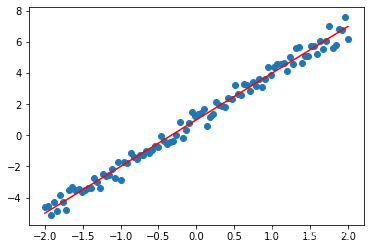
plt.scatter(x,y)
plt.plot(x,3*x+1,'r')
plt.plot(x,w.numpy()*x+b.numpy(),'y')

[<matplotlib.lines.Line2D at 0x7f54c4852dd8>]

# 查看损失
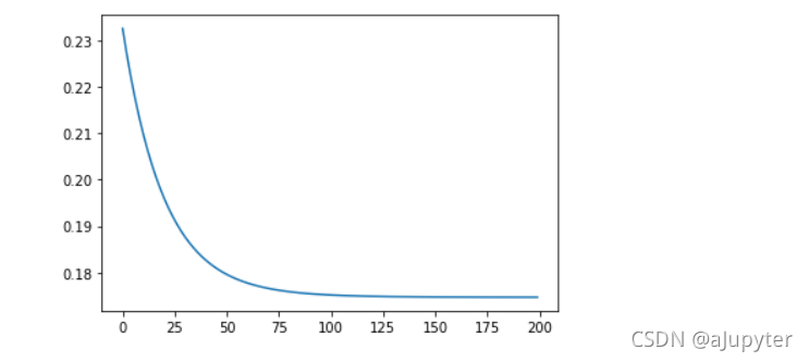
plt.plot(loss_list)

[<matplotlib.lines.Line2D at 0x7f54c4868f60>]

三、预测

model(2,w.numpy(),b.numpy()).numpy()

6.9262376

BGD

for epoch in range(training_epochs):
        # 梯度下降
        # 1.计算梯度
        loss_list.append(loss(x,y,w,b))
        delta_w,delta_b = grand(x,y,w,b)
        # 2.梯度下降
        w_change = delta_w * learning_rate
        b_change = delta_b * learning_rate
        w.assign_sub(w_change)
        b.assign_sub(b_change)

# 查看损失
plt.plot(loss_list)