import numpy as np
import matplotlib.pyplot as plt
from sklearn.pipeline import Pipeline
from sklearn.preprocessing import PolynomialFeatures
from sklearn.linear_model import LinearRegression
from sklearn.model_selection import cross_val_score
%matplotlib inline
def true_fun (X) :return np.cos(1.5 * np.pi * X)
np.random.seed(0 )
n_samples = 30
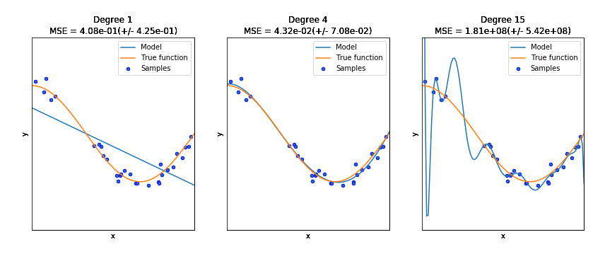
degrees = [1 , 4 , 15 ]
X = np.sort(np.random.rand(n_samples))
y = true_fun(X) + np.random.randn(n_samples) * 0.1
print(X.shape,y.shape)
print()
print(X)
print()
print(y)
(30,) (30,)

[0.0202184  0.07103606 0.0871293  0.11827443 0.14335329 0.38344152
 0.41466194 0.4236548  0.43758721 0.46147936 0.52184832 0.52889492
 0.54488318 0.5488135  0.56804456 0.60276338 0.63992102 0.64589411
 0.71518937 0.77815675 0.78052918 0.79172504 0.79915856 0.83261985
 0.87001215 0.891773   0.92559664 0.94466892 0.96366276 0.97861834]

[ 1.0819082   0.87027612  1.14386208  0.70322051  0.78494746 -0.25265944
 -0.22066063 -0.26595867 -0.4562644  -0.53001927 -0.86481449 -0.99462675
 -0.87458603 -0.83407054 -0.77090649 -0.83476183 -1.03080067 -1.02544303
 -1.0788268  -1.00713288 -1.03009698 -0.63623922 -0.86230652 -0.75328767
 -0.70023795 -0.41043495 -0.50486767 -0.27907117 -0.25994628 -0.06189804]
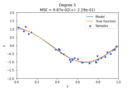
degree=5
polynomial_features = PolynomialFeatures(degree=degree,include_bias=False )
linear_regression = LinearRegression()
pipeline = Pipeline([("polynomial_features" , polynomial_features),("linear_regression" , linear_regression)])
pipeline.fit(X[:, np.newaxis], y)
scores = cross_val_score(pipeline, X[:, np.newaxis], y,scoring="neg_mean_squared_error" , cv=10 )
X_test = np.linspace(0 , 1 , 100 )
plt.plot(X_test, pipeline.predict(X_test[:, np.newaxis]), label="Model" )
plt.plot(X_test, true_fun(X_test), label="True function" )
plt.scatter(X, y, edgecolor='b' , s=20 , label="Samples" )
plt.xlabel("x" )
plt.ylabel("y" )
plt.xlim((0 , 1 ))
plt.ylim((-2 , 2 ))
plt.legend(loc="best" )
plt.title("Degree {}\nMSE = {:.2e}(+/- {:.2e})" .format(degree, -scores.mean(), scores.std()))
Text(0.5, 1.0, 'Degree 5\nMSE = 9.87e-02(+/- 2.29e-01)')
plt.figure(figsize=(14 , 5 ))
for i in range(len(degrees)):
ax = plt.subplot(1 , len(degrees), i + 1 )
plt.setp(ax, xticks=(), yticks=())
polynomial_features = PolynomialFeatures(degree=degrees[i],include_bias=False )
linear_regression = LinearRegression()
pipeline = Pipeline([("polynomial_features" , polynomial_features),
("linear_regression" , linear_regression)])
pipeline.fit(X[:, np.newaxis], y)
scores = cross_val_score(pipeline, X[:, np.newaxis], y,
scoring="neg_mean_squared_error" , cv=10 )
X_test = np.linspace(0 , 1 , 100 )
plt.plot(X_test, pipeline.predict(X_test[:, np.newaxis]), label="Model" )
plt.plot(X_test, true_fun(X_test), label="True function" )
plt.scatter(X, y, edgecolor='b' , s=20 , label="Samples" )
plt.xlabel("x" )
plt.ylabel("y" )
plt.xlim((0 , 1 ))
plt.ylim((-2 , 2 ))
plt.legend(loc="best" )
plt.title("Degree {}\nMSE = {:.2e}(+/- {:.2e})" .format(degrees[i], -scores.mean(), scores.std()))
plt.show()
分类器
导入必要的包、读入数据
import pandas as pd
import numpy as np
import matplotlib.pyplot as plt
from pandas import Series, DataFrame
from scipy import stats
%matplotlib inline
mydata=pd.read_excel('./CLFData/个人收入水平调查分析.xlsx' )
mydata.head(100 )
年龄
受教育时间
性别
资产净增
资产损失
一周工作时间
收入水平
0
39
13
Male
2174
0
40
<=50K
1
50
13
Male
0
0
13
<=50K
2
38
9
Male
0
0
40
<=50K
3
53
7
Male
0
0
40
<=50K
4
28
13
Female
0
0
40
<=50K
...
...
...
...
...
...
...
...
95
29
10
Male
0
0
50
<=50K
96
48
16
Male
0
1902
60
>50K
97
37
10
Male
0
0
48
>50K
98
48
12
Female
0
0
40
<=50K
99
32
9
Male
0
0
40
<=50K
100 rows × 7 columns
检查数据缺失度
mydata.info()
<class 'pandas.core.frame.DataFrame'>
RangeIndex: 32561 entries, 0 to 32560
Data columns (total 7 columns):
 #   Column  Non-Null Count  Dtype
---  ------  --------------  -----
 0   年龄      32561 non-null  int64
 1   受教育时间   32561 non-null  int64
 2   性别      32561 non-null  object
 3   资产净增    32561 non-null  int64
 4   资产损失    32561 non-null  int64
 5   一周工作时间  32561 non-null  int64
 6   收入水平    32561 non-null  object
dtypes: int64(5), object(2)
memory usage: 1.7+ MB
变量类型处理
mydata.describe()
mydata['性别' ]=mydata['性别' ].map( {'Female' : 1 , 'Male' : 0 } ).astype(int)
mydata['收入水平' ]=mydata['收入水平' ].map( {'>50K' : 1 , '<=50K' : 0 } ).astype(int)
mydata.head()
年龄
受教育时间
性别
资产净增
资产损失
一周工作时间
收入水平
0
39
13
0
2174
0
40
0
1
50
13
0
0
0
13
0
2
38
9
0
0
0
40
0
3
53
7
0
0
0
40
0
4
28
13
1
0
0
40
0
分割自变量和因变量
X=mydata.drop(['收入水平' ],axis=1 )
X
年龄
受教育时间
性别
资产净增
资产损失
一周工作时间
0
39
13
0
2174
0
40
1
50
13
0
0
0
13
2
38
9
0
0
0
40
3
53
7
0
0
0
40
4
28
13
1
0
0
40
...
...
...
...
...
...
...
32556
27
12
1
0
0
38
32557
40
9
0
0
0
40
32558
58
9
1
0
0
40
32559
22
9
0
0
0
20
32560
52
9
1
15024
0
40
32561 rows × 6 columns
y=mydata['收入水平' ]
X.shape,y.shape
((32561, 6), (32561,))
from sklearn.model_selection import train_test_split
X_train,X_test,y_train,y_test=train_test_split(X,y,random_state=4 )
X_train.shape,X_test.shape,y_train.shape,y_test.shape
((24420, 6), (8141, 6), (24420,), (8141,))
决策树C4.5
from sklearn import tree
clf=tree.DecisionTreeClassifier()
clf.fit(X,y)
print(clf.predict(X))
print('准确率:' ,1 -(clf.predict(X)!=y).sum()/len(y))
y_pred_dt=clf.predict(X)
from sklearn import metrics
print(metrics.classification_report(y,y_pred_dt))
print(metrics.confusion_matrix(y,y_pred_dt))
print(metrics.f1_score(y,y_pred_dt))
[0 0 0 ... 0 0 1]
准确率: 0.8955806025613464
              precision    recall  f1-score   support

           0       0.90      0.97      0.93     24720
           1       0.89      0.65      0.75      7841

    accuracy                           0.90     32561
   macro avg       0.89      0.81      0.84     32561
weighted avg       0.90      0.90      0.89     32561

[[24097   623]
 [ 2777  5064]]
0.7486694263749261
from sklearn import tree
clf=tree.DecisionTreeClassifier()
clf.fit(X_train,y_train)
print(clf.predict(X_train))
print('准确率:' ,1 -(clf.predict(X_train)!=y_train).sum()/len(y_train))
y_test_pred_dt=clf.predict(X_test)
from sklearn import metrics
print(metrics.classification_report(y_test,y_test_pred_dt))
print(metrics.confusion_matrix(y_test,y_test_pred_dt))
print(metrics.f1_score(y_test,y_test_pred_dt))
[0 0 0 ... 0 1 0]
准确率: 0.8997952497952498
              precision    recall  f1-score   support

           0       0.86      0.91      0.88      6172
           1       0.66      0.51      0.58      1969

    accuracy                           0.82      8141
   macro avg       0.76      0.71      0.73      8141
weighted avg       0.81      0.82      0.81      8141

[[5647  525]
 [ 957 1012]]
0.5772960638904735
KNN
from sklearn.neighbors import KNeighborsClassifier
clf=KNeighborsClassifier(n_neighbors=3 )
clf.fit(X,y)
print(clf.predict(X))
print('准确率:' ,1 -(clf.predict(X)!=y).sum()/len(y))
y_pred_knn=clf.predict(X)
from sklearn import metrics
print(metrics.classification_report(y,y_pred_knn))
print(metrics.confusion_matrix(y,y_pred_knn))
print(metrics.f1_score(y,y_pred_knn))
[0 0 1 ... 0 0 1]
准确率: 0.8591259482202636
              precision    recall  f1-score   support

           0       0.89      0.93      0.91     24720
           1       0.74      0.64      0.69      7841

    accuracy                           0.86     32561
   macro avg       0.82      0.78      0.80     32561
weighted avg       0.85      0.86      0.86     32561

[[22947  1773]
 [ 2814  5027]]
0.6867017280240421
from sklearn.neighbors import KNeighborsClassifier
clf=KNeighborsClassifier(n_neighbors=3 )
clf.fit(X_train,y_train)
print(clf.predict(X_train))
print('准确率:' ,1 -(clf.predict(X_train)!=y_train).sum()/len(y_train))
y_test_pred_knn=clf.predict(X_test)
from sklearn import metrics
print(metrics.classification_report(y_test,y_test_pred_knn))
print(metrics.confusion_matrix(y_test,y_test_pred_knn))
print(metrics.f1_score(y_test,y_test_pred_knn))
[0 0 0 ... 0 1 0]
准确率: 0.8949356592242252
              precision    recall  f1-score   support

           0       0.87      0.90      0.88      6172
           1       0.63      0.56      0.60      1969

    accuracy                           0.82      8141
   macro avg       0.75      0.73      0.74      8141
weighted avg       0.81      0.82      0.81      8141

[[5533  639]
 [ 858 1111]]
0.5974724388276419
逻辑回归
from sklearn.linear_model import LogisticRegression
clf=LogisticRegression(max_iter=200 )
clf.fit(X,y)
print(clf.predict(X))
print('准确率:' ,1 -(clf.predict(X)!=y).sum()/len(y))
y_pred_log=clf.predict(X)
from sklearn import metrics
print(metrics.classification_report(y,y_pred_log))
print(metrics.confusion_matrix(y,y_pred_log))
print(metrics.f1_score(y,y_pred_log))
[1 0 0 ... 0 0 1]
准确率: 0.8225177359417708
              precision    recall  f1-score   support

           0       0.84      0.95      0.89     24720
           1       0.72      0.43      0.54      7841

    accuracy                           0.82     32561
   macro avg       0.78      0.69      0.72     32561
weighted avg       0.81      0.82      0.81     32561

[[23384  1336]
 [ 4443  3398]]
0.5404373757455269
from sklearn.linear_model import LogisticRegression
clf=LogisticRegression(max_iter=200 )
clf.fit(X_train,y_train)
print(clf.predict(X_train))
print('准确率:' ,1 -(clf.predict(X_train)!=y_train).sum()/len(y_train))
y_test_pred_log=clf.predict(X_test)
from sklearn import metrics
print(metrics.classification_report(y_test,y_test_pred_log))
print(metrics.confusion_matrix(y_test,y_test_pred_log))
print(metrics.f1_score(y_test,y_test_pred_log))
[0 0 0 ... 0 1 0]
准确率: 0.8215397215397215
              precision    recall  f1-score   support

           0       0.84      0.94      0.89      6172
           1       0.72      0.45      0.56      1969

    accuracy                           0.82      8141
   macro avg       0.78      0.70      0.72      8141
weighted avg       0.81      0.82      0.81      8141

[[5822  350]
 [1075  894]]
0.5564892623716153
clf
LogisticRegression(C=1.0, class_weight=None, dual=False, fit_intercept=True,
                   intercept_scaling=1, l1_ratio=None, max_iter=100,
                   multi_class='auto', n_jobs=None, penalty='l2',
                   random_state=None, solver='lbfgs', tol=0.0001, verbose=0,
                   warm_start=False)
"""
y_pred=clf.predict(X)
from sklearn import metrics
print(metrics.classification_report(y,y_pred))
print(metrics.confusion_matrix(y,y_pred))
"""
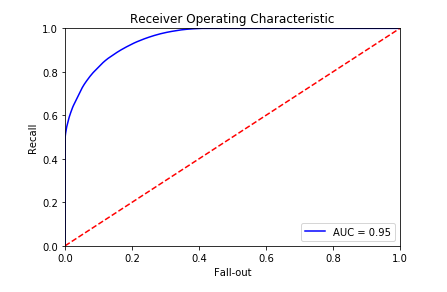
from sklearn.metrics import roc_curve, auc,confusion_matrix,precision_score ,recall_score,f1_score
predictions = clf.predict_proba(X_test)
false_positive_rate, recall, thresholds = roc_curve(y, predictions[:, 1 ])
roc_auc = auc(false_positive_rate, recall)
plt.title('Receiver Operating Characteristic' )
plt.plot(false_positive_rate, recall, 'b' , label='AUC = %0.2f' % roc_auc)
plt.legend(loc='lower right' )
plt.plot([0 , 1 ], [0 , 1 ], 'r--' )
plt.xlim([0.0 , 1.0 ])
plt.ylim([0.0 , 1.0 ])
plt.ylabel('Recall' )
plt.xlabel('Fall-out' )
plt.show()