

1.提出问题
根据提供的相关数据建模预测房价。
2.数据来源及理解
(1)数据来源:kaggle(www.kaggle.com/c/house-pri…)
(2)数据指标:变量很多有81个,要在分析实际情况的基础上加上理论分析,选择跟目标相关性强的变量进行数据分析。
3.数据清洗
#导入要用的模块
import pandas as pd
import matplotlib.pyplot as plt
import numpy as py
import seaborn as sns
from scipy import stats
from scipy.stats import norm
from sklearn.preprocessing import StandardScaler
#忽略警告
import warnings
warnings.filterwarnings('ignore')

#导入数据
train=pd.read_csv('C:/Users/雪小玲/Desktop/项目/house-price/train.csv')
print(train.shape)
#结果:
(1460, 81)
(一)查看目标变量:有无缺失值?描述性统计情况如何?
print(train['SalePrice'].describe())
#结果:
count      1460.000000
mean     180921.195890
std       79442.502883
min       34900.000000
25%      129975.000000
50%      163000.000000
75%      214000.000000
max      755000.000000
Name: SalePrice, dtype: float64
#无缺失值或无效数据,进一步查看数据分布情况
sns.distplot(train['SalePrice'])
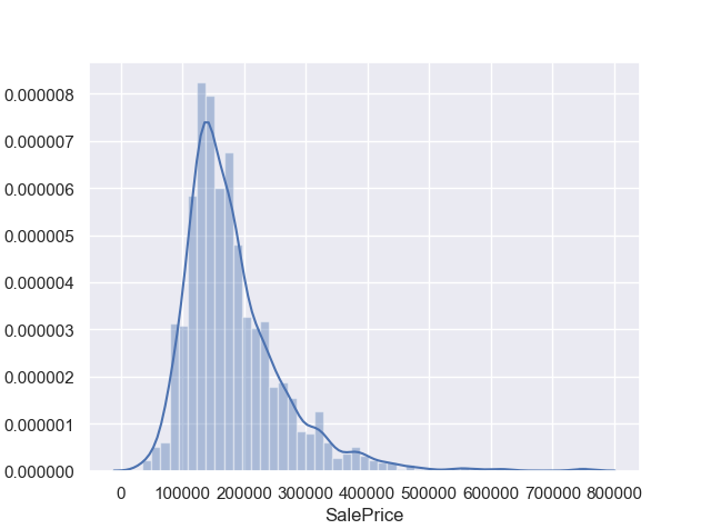
print('Skewness:%f'%train['SalePrice'].skew())
print('Kurtosis:%f'%train['SalePrice'].kurt())
#结果:
Skewness:1.882876
Kurtosis:6.536282

#根据偏度S=1.8和峰度K=6.5可知,SalePrice呈右偏尖峰分布,后续可考虑对数变换
(二)分析特征数据和目标变量:箱形图/散点图
#(1)理论入选特征变量
#Utilities:一般居家设施越齐全房价会越贵,但是基本全部都是AllPub——设施齐备,不考虑
#LotArea:面积越大房价越贵,数据不同,考虑
#Neighborhood:所处地理位置位置,考虑
#OverallQual:房屋整体评估,考虑
#YearBuilt:建造年份,考虑
#TotalBsmtSF & GrLivArea:很多涉及面积的变量,简化TotalBsmtSF(地下室面积)和GrLivArea(不含车库的室内面积)
#Heating:供暖方式,基本都是GasA,不考虑
#CentralAir:中央空调,考虑
#MiscVal:价格分档次0-3500之间,考虑
#GarageCars & GarageArea:存放车辆数和车库面积,数据不同,考虑

#(2)验证入选的变量是否合理
#分类型变量:
#1.地理位置Neighborhood
var1='Neighborhood'
data1=pd.concat([train['SalePrice'],train[var1]],axis=1)
f,ax=plt.subplots(figsize=(26,12))
fig1=sns.boxplot(x=var1,y='SalePrice',data=data1)
fig1.axis(ymin=0,ymax=800000)
fig1.grid(axis='y')
plt.show()
#箱线图可以看出,位置不同的房屋价格不同
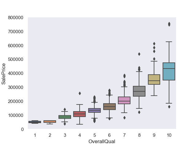
#2.房屋整体评估OverallQual
var2='OverallQual'
data2=pd.concat([train['SalePrice'],train[var2]],axis=1)
fig2=sns.boxplot(x=var2,y='SalePrice',data=data2)
fig2.axis(ymin=0,ymax=800000)
fig2.grid(axis='y')
plt.show()
#箱线图可以看出,整体评价越高的房屋价格越高
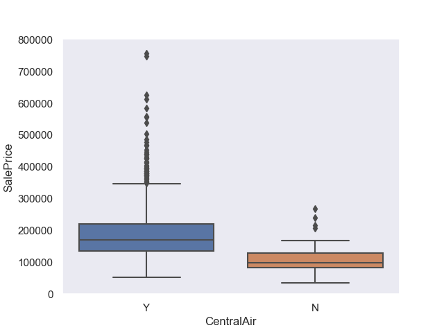
#3.中央空调CentralAir
var3='CentralAir'
data3=pd.concat([train['SalePrice'],train[var3]],axis=1)
fig3=sns.boxplot(x=var3,y='SalePrice',data=data3)
fig3.axis(ymin=0,ymax=800000)
fig3.grid(axis='y')
plt.show()
#箱形图可以看出,有中央空调的房屋价格更高

#数值型变量
#1.建造年份YearBuilt
var4='YearBuilt'
data4=pd.concat([train['SalePrice'],train[var4]],axis=1)
data4.plot.scatter(x=var4,y='SalePrice',ylim=(0,800000))
plt.show()
#可见,随着建造年份越晚,房价越高

#2.占地面积LotArea
var5='LotArea'
data5=pd.concat([train['SalePrice'],train[var5]],axis=1)
data5.plot.scatter(x=var5,y='SalePrice',ylim=(0,800000))
plt.show()
#价格随面积越高而越高,但不是很明显

#3.不含车库的室内面积GrLivArea
var6='GrLivArea'
data6=pd.concat([train['SalePrice'],train[var6]],axis=1)
data6.plot.scatter(x=var6,y='SalePrice',ylim=(0,800000))
plt.show()
#明显,房价随面积增大而越高

#4.地下室面积TotalBsmtSF
var7='TotalBsmtSF'
data7=pd.concat([train['SalePrice'],train[var7]],axis=1)
data7.plot.scatter(x=var7,y='SalePrice',ylim=(0,800000))
plt.show()
#明显,房价随面积增大而越高

#5.附加资产MiscVal
var8='MiscVal'
data8=pd.concat([train['SalePrice'],train[var8]],axis=1)
data8.plot.scatter(x=var8,y='SalePrice',ylim=(0,800000))
plt.show()
#可以看出,附加资产对房价没很明显的影响,可以排除

#6.车库面积和车库车辆GarageCars/GarageArea
vars9=['GarageCars','GarageArea']
for var in vars9:
    data9=pd.concat([train['SalePrice'],train[var]],axis=1)
    data9.plot.scatter(x=var,y='SalePrice',ylim=(0,800000))
    plt.show()
#可以看出,随车库面积/车库车辆数的增大房价会增高
#综上,入选的变量有:Neighborhood、OverallQual、CentralAir、YearBuilt、LotArea、GrLivArea、TotalBsmtSF、GarageCars/GarageArea
(三)所有变量的关系研究:特征关系矩阵、目标变量的关系矩阵、关系图
#1.关系矩阵-热力图
f,ax=plt.subplots(figsize=(20,9))
sns.heatmap(train.corr(),vmax=0.8,square=True)
#可以看出各变量与SalePrice的关系:
#OverallQual整体评估、TotalBsmtSF地下室总面积、1stFlrSF一楼面积、GrLivArea不含车库的室内面积、GarageCars/GarageArea车库面积相关性很强
#YearBuilt建造年份、FullBath带浴缸的浴室、TotRmsAbvGrd总房间数相关性较弱

#2.上述颜色观察不够准确,类似特征需要做出取舍,还有分类型数据要讨论
#不以连续值的形式给出,如性别、国家等采用OnehotEncoder,表示不同取值间的差异一样;对于离散的数值或文本,可采用LabelEncoder编码。
#离散型数据,Neighborhood等
from sklearn import preprocessing
f_names=['CentralAir','Neighborhood']
for x in f_names:
    label=preprocessing.LabelEncoder()
    train[x]=label.fit_transform(train[x])
corrmat=train.corr()
f,ax=plt.subplots(figsize=(20,9))
sns.heatmap(corrmat,vmax=0.8,square=True)
#可以看到,两者跟目标变量的相关性不大,舍弃

#3.取相关性最大的变量,画关系矩阵图
k=10
cols=corrmat.nlargest(k,'SalePrice')['SalePrice'].index
cm=np.corrcoef(train[cols].values.T)
sns.set(font_scale=1.25)
hm=sns.heatmap(cm,cbar=True,annot=True,square=True,
    fmt='.2f',annot_kws={'size':10},yticklabels=cols.values,xticklabels=cols.values)
plt.show()
#由图可知,OverallQual、GrLivArea的相关性最强,选取
#GarageCars和GarageArea相近,选取相关性更强的前者
#TotalBsmtSF(地下室总面积)和1stFlrSF(一楼面积)类似,选取前者
#FullBath选取
#TotRmsAbvGrd(总房间数)和GrLivArea(地上居住面积)类似,YearBuilt,都选取

#绘制关系图
sns.set()
cols=['SalePrice','OverallQual','GrLivArea','GarageCars','TotalBsmtSF','1stFlrSF','FullBath','TotRmsAbvGrd','YearBuilt']
sns.pairplot(train[cols],size=2.5)
plt.show()
4.构建模型
(一)构建模型并评价
from sklearn import preprocessing
from sklearn import linear_model,svm,gaussian_process
from sklearn.ensemble import RandomForestRegressor
from sklearn.model_select import train_test_split
cols=['OverallQual','GrLivArea','GarageCars','TotalBsmtSF','1stFlrSF','FullBath','TotRmsAbvGrd','YearBuilt']
x=train[cols].values
y=train['SalePrice'].values
#归一化处理之后,模型模拟并计算各自的误差
x_scale=preprocessing.StandardScaler().fit_transform(x)
y_scale=preprocessing.StandardScaler().fit_transform(y.reshape(-1,1))
x_train,x_test,y_train,y_test=train_test_split(x_scale,y_scale,test_size=0.33,random_state=42)
clfs={'svm':svm.SVR(),
      'Rand_For_Reg':RandomForestRegressor(n_estimators=400),
      'Bay_Rid':linear_model.BayesianRidge()}
for clf in clfs:
    try:
    clfs[clf].fit(x_train,y_train)
    y_pred=clfs[clf].predict(x_test)
    print(clf+'cost'+str(np.sum(y_pred-y_test)/len(y_pred)))
    except Exception as e:
    print(clf+'Error')
    print(str(e))
(二)随机森林模型的效果最好,不进行归一化的模型查看效果
clf=RandomForestRegressor(n_estimators=400)
clf.fit(x_train,y_train)
y_pred=clf.predict(x_test)
#保留模型的参数
rfr=clf
print(str(np.sum(abs(y_pred-y_test)/len(y_pred))))
(三)用该模型进行预测
import pandas as pd
from sklearn.ensemble import RandomForestRegressor
test=pd.read_csv('C:/Users/雪小玲/Desktop/项目/house-price/test.csv')
#查看数据,存在缺失值,不能直接预测
print(test[cols].info())
#GarageCars和TotalBsmtSF均有一个缺失值,用均值补充
test['GarageCars']=test['GarageCars'].fillna(round(test['GarageCars'].mean(),2))
test['TotalBsmtSF']=test['TotalBsmtSF'].fillna(test['TotalBsmtSF'].mean())
test_x=test[cols]
print(test_x.isnull().sum())
x=test_x.values
y_test_pred=rfr.predict(x)
print(x.shape,y_test_pred.shape)
prediction=pd.DataFrame(y_test_pred,columns=['SalePrice'])
result=pd.concat([test['Id'],prediction],axis=1)
print(result.columns)
#保存结果
result.to_csv('C:/Users/雪小玲/Desktop/项目/house-price/prediction.csv',index=False')
