If in the deterministic case, the adjoint equations are backward ordinary differential equations and represent, in some sense, the same forward equation.

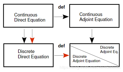
Continuous vs. Discrete Adjoint Equations

The adjoint equations can be derived using two different approaches.

By definition we have

Both with advantages and disadvantages:

Continuous approach: The adjoint equations are derived by definition using the continuous direct equations.

+ Straightforward derivation, reuse old code when programming;
– Accuracy depends on discretization, difficulties with boundary conditions.

Discrete approach: The adjoint equations are derived from the discretized direct equations.

+ Accuracy can be achieved close to machine precision,and can be independent of discretization;
–Tricky derivation, usually requires making a new code,or larger changes of an existing code.

Here " def " means definition of the adjoint operator.

Consider the following optimization problem (ODE) whereφis the state andgthe control

{\frac{d\phi(t)}{dt}}=−A\phi(t) +Bg(t), for \ 0≤t≤T,

with initial condition

We can now define an optimization problem in which the goal is to find an optimalg(t) by minimizing the following objective function

J={\frac{γ_{1}}{2}}[\phi(T)−Ψ]^2+{\frac{γ_{2}}{2}}\int_0^T g(t)^2dt,

Continuous approach

We can solve this problem using an adjoint identity approach or by introducing Lagrange multipliers.

\int_0^T a[{\frac{d\phi}{dt}}+A\phi−Bg]dt=\int_0^T[-{\frac{da}{dt}}+A^∗a]\phi dt−\int_0^T aBg dt+a(T)\phi(T)−a(0)\phi(0).

If we now define the adjoint equation as $−{\frac{da}{dt}}=−A∗a$ with an arbitrary initial condition $a(T)$ then the identity reduces to:

LHS =−\int_0^TaBg dt+a(T)\phi(T)−a(0)\phi(0)

By definition the Left Hand Side is identically zero but this is exactly what must be checked numerically , i.e. error=|LHS|.

The gradient of Jw.r.t. g can be derived considering the J is nonlinear in $\phi$ and $g$ . We linearise by $\phi→\phi+δ\phi$ , $g→g+δg$ and then write the linearised objective function as:

γ_{1}[\phi(T)−Ψ]δ\phi(T) =δJ−γ_{2}\int_0^Tgδg dt,

If we choose $a(T) =γ_{1}[\phi(T)−Ψ]$ then the equation for $δJ$ can be substituted into the expression for the adjoint identity. If you further define the adjoint equations, remember that $δ\phi(0) = 0$ , then the final identity is written：

The adjoint equations and gradient of Jw.r.t. g are written:

−{\frac{da}{dt}}+A^∗a, \quad a(T) =γ_{1}[\phi(T)−Ψ], \quad and \quad ∇Jg=γ_{2}g+B^∗a.

The so called optimality condition is given by $∇Jg= 0$ .

Discrete approach

A discrete version of the direct equation is written：

{\frac{\phi^{i+1}−\phi^i}{∆t}}=−A\phi^i+Bg^i,\quad fori= 1,...,N−1,

where $N$ denotes the number of discrete points on the interval $[0,T]$ , $∆t$ is the constant time step, and

is the initial condition. This can be written as a discrete evolution equation.

\phi^{i+1}=L\phi^i+ ∆t Bg^i,\quad for i= 1,...,N−1.

with $L=I−∆tA$ , and $I$ the identity matrix. A discrete version of the objective function can be written:

J={\frac{γ_{1}}{2}}(\phi N−Φ)^2+{\frac{γ_{2}}{2}}\sum\limits_{i=1}^{N-1} ∆t(g^i)^2.

An adjoint variable $a^i$ is introduced defined on $i= 1,...,N$ and we write the adjoint identity as

a^{i+1}·L\phi^i= (L^*a^{i+1})·\phi^i, \quad for \quad i= 1,...,N−1.

We then introduce the definition of the state equation on the left hand side of and impose that

a^i=L^*a^{i+1} \quad for\quad i=N−1,...,1

This is thediscrete adjoint equation. Using the discrete direct and adjoint yields:

a^{i+1}·(\phi^{i+1}−∆tBg^i) =a^i·φ^i,\quad for\quad i= 1,...,N−1

which must be valid for any $\phi$ and $a$ . An error can therefore be written as

error =|a^N·\phi^N−a^1·\phi^1−\sum\limits_{i=1}^{N-1}∆t a^{i+1}·Bg^i|.

This can be compared with the error for the continuous formulation from the previous derivation

error =|a(T)\phi(T)−a(0)\phi(0)−\int_0^T aBg dt|

Comparison

Error from the discrete approach

Error from the continuous approach

The convergence of the physical problem and the accuracy of the gradient can be considered two different issues.

In the continuous approach the adjoint solution depends on the discretization scheme used and the error will decrease as the spatial and temporal resolution increase. In this case it is difficult to distinguish between different errors in the case an optimization problem fail to converge.
The advantage of the discrete approach is that the adjoint solution will be numerically "exact", independently of the spatial and temporal resolution.

The discrete optimality condition is then derived. Since $J$ is nonlinear with respect to $\phi$ and $g$ we must first linearize. This can be written

δJ=γ_{1}(φ^N−Φ)·δ\phi^N+γ_{2}\sum\limits_{i=1}^{N-1}∆tg^i·δg^i.

We now choose the terminal condition of the adjoint as $a^N=γ_{1}(\phi^N−Φ)$ and substitute this expression into the discrete adjoint identity. This is written

γ_{1}(\phi^N−Φ)·δ\phi^N=a^1·δ\phi^1+\sum\limits_{i=1}^{N-1}∆t a^{i+1}·Bδg^i

By inspection one can see that the left hand side is identical to the first term in the expression for $δJ$ , and $δ\phi^1= 0$ . Rearranging the terms, we get

δJ=\sum\limits_{i=1}^{N-1}∆t(γ_{2}g^i+B^*a^{i+1})·δg^i,

from which we get the discrete optimality condition

g^i=−{\frac{1}{γ_{2}}}B^*a^{i+1} \quad for \quad i= 1,..,N−1.

Note that if $B$ is a matrix then $B^*=B^T$

Derivation of the adjoint equation

Continuous vs. Discrete Adjoint Equations

Continuous approach

Discrete approach

Comparison