

欢迎转载转发,但请标明出处,源码、notebook以及最新内容请访问:github.com/zhulei227/M…
from imblearn_utils import *
from sklearn.datasets import make_classification
import numpy as np
import warnings
warnings.filterwarnings("ignore")
import matplotlib.pyplot as plt
%matplotlib inline
这一节关注不同的影响因素对不同分类模型的影响,在这之前,首先需要介绍对不平衡分类比较合理的性能评估指标,常用的是这三项,这里对
单独说一下,它是各类准确率的几何平均:
这里,表示类别数,
表示第
类的准确率,特别地,对于二分类有
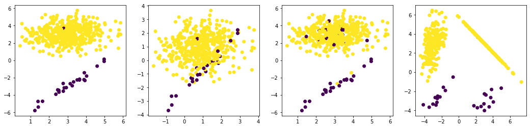
接下来,利用上一节的4类数据(类间不平衡,数据交叠,异常点、类内不平衡)对一些常用的模型进行建模,并比较这三项指标的变化,主要进行比较的模型包括lr,nb,svm,rf,gbdt这几种
#sklearn中没有对G_{mean}的计算,这里定义一个
def g_score(y_true,y_pre):
    y_set=set(y_true)
    accs=[]
    for y_label in y_set:
        accs.append(np.sum((y_true==y_label)*(y_pre==y_label))/np.sum(y_true==y_label))
    g_score=1.0
    for acc in accs:
        g_score*=acc
    return np.power(g_score,1.0/len(accs))
#造数据
n_samples=500
X1, y1 = make_classification(n_samples=n_samples, n_features=2,
                           n_informative=2,n_redundant=0,
                           n_repeated=0, n_classes=2,
                           n_clusters_per_class=1,weights=[0.05, 0.95],
                           class_sep=3, random_state=0)
X2, y2 = make_classification(n_samples=n_samples, n_features=2,
                           n_informative=2,n_redundant=0,
                           n_repeated=0, n_classes=2,
                           n_clusters_per_class=1,weights=[0.05, 0.95],
                           class_sep=0.9, random_state=0)
X3, y3 = make_classification(n_samples=n_samples, n_features=2,
                           n_informative=2,n_redundant=0,
                           n_repeated=0, n_classes=2,
                           n_clusters_per_class=1,weights=[0.05, 0.95],
                           class_sep=3,flip_y=0.1, random_state=0)
X4, y4 = make_classification(n_samples=n_samples, n_features=2,
                           n_informative=2,n_redundant=0,
                           n_repeated=0, n_classes=2,
                           n_clusters_per_class=2,weights=[0.05, 0.95],
                           class_sep=3.0,random_state=0)
plt.figure(figsize = (18,4))
plt.subplot(1,4,1)
plt.scatter(x=X1[:,0],y=X1[:,1],c=y1)
plt.subplot(1,4,2)
plt.scatter(x=X2[:,0],y=X2[:,1],c=y2)
plt.subplot(1,4,3)
plt.scatter(x=X3[:,0],y=X3[:,1],c=y3)
plt.subplot(1,4,4)
plt.scatter(x=X4[:,0],y=X4[:,1],c=y4)
<matplotlib.collections.PathCollection at 0x16f47e1d908>
#导入模型
from sklearn.linear_model import LogisticRegression
from sklearn.svm import SVC
from sklearn.ensemble import RandomForestClassifier
from sklearn.ensemble import GradientBoostingClassifier
from sklearn.model_selection import train_test_split
from sklearn.metrics import roc_auc_score,f1_score
#封装训练过程并返回指标
def train(Model,X,y):
    if Model.__name__=="SVC":
        model=Model(probability=True)
    else:
        model=Model()
    X_train,X_test,y_train,y_test=train_test_split(X,y,test_size=0.2, random_state=0)
    model.fit(X_train,y_train)
    y_pred=model.predict(X_test)
    y_pred_proba=model.predict_proba(X_test)
    return model,f1_score(y_test,y_pred,average='macro'),g_score(y_test,y_pred),roc_auc_score(y_test,y_pred_proba[:,1],average="macro")
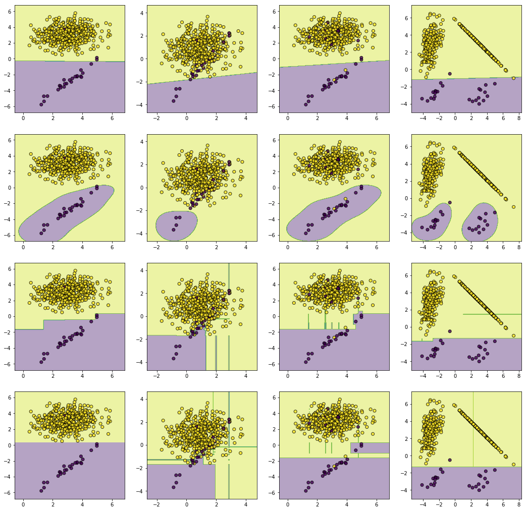
#定义决策边界绘图函数
#copy from:https://imbalanced-learn.org/stable/auto_examples/under-sampling/plot_comparison_under_sampling.html#sphx-glr-auto-examples-under-sampling-plot-comparison-under-sampling-py
def plot_decision_function(X, y, clf, plt):
    plot_step = 0.02
    x_min, x_max = X[:, 0].min() - 1, X[:, 0].max() + 1
    y_min, y_max = X[:, 1].min() - 1, X[:, 1].max() + 1
    xx, yy = np.meshgrid(np.arange(x_min, x_max, plot_step),
                         np.arange(y_min, y_max, plot_step))

    Z = clf.predict(np.c_[xx.ravel(), yy.ravel()])
    Z = Z.reshape(xx.shape)
    plt.contourf(xx, yy, Z, alpha=0.4)
    plt.scatter(X[:, 0], X[:, 1], alpha=0.8, c=y, edgecolor='k')
#训练
plt.figure(figsize = (18,18))
f1_scores=[]
g_scores=[]
aucs=[]
for i,Model in enumerate([LogisticRegression,SVC,RandomForestClassifier,GradientBoostingClassifier]):
    model_name=Model.__name__
    tmp_f1=[model_name]
    tmp_g=[model_name]
    tmp_auc=[model_name]
    for j,(X,y) in enumerate([(X1,y1),(X2,y2),(X3,y3),(X4,y4)]):
        model,f1,g,auc=train(Model,X,y)
        tmp_f1.append(f1)
        tmp_g.append(g)
        tmp_auc.append(auc)
        plt.subplot(4,4,i*4+j+1)
        plot_decision_function(X,y,model,plt)
    f1_scores.append(tmp_f1)
    g_scores.append(tmp_g)
    aucs.append(tmp_auc)
import pandas as pd
f1_df=pd.DataFrame(f1_scores,columns=['分类器名称','类间不平衡','数据重叠','异常值','类内不平衡'])
g_df=pd.DataFrame(g_scores,columns=['分类器名称','类间不平衡','数据重叠','异常值','类内不平衡'])
auc_df=pd.DataFrame(aucs,columns=['分类器名称','类间不平衡','数据重叠','异常值','类内不平衡'])
#f1值对比
f1_df
| 分类器名称 | 类间不平衡 | 数据重叠 | 异常值 | 类内不平衡 | |
|---|---|---|---|---|---|
| 0 | LogisticRegression | 0.938950 | 0.56710 | 0.789474 | 0.9519 |
| 1 | SVC | 0.970922 | 0.56710 | 0.855700 | 0.9519 |
| 2 | RandomForestClassifier | 0.970922 | 0.69278 | 0.794323 | 0.9519 |
| 3 | GradientBoostingClassifier | 0.970922 | 0.69278 | 0.822695 | 0.9519 |
#g值对比
g_df
| 分类器名称 | 类间不平衡 | 数据重叠 | 异常值 | 类内不平衡 | |
|---|---|---|---|---|---|
| 0 | LogisticRegression | 0.894427 | 0.316228 | 0.703336 | 0.912871 |
| 1 | SVC | 0.948683 | 0.316228 | 0.812142 | 0.912871 |
| 2 | RandomForestClassifier | 0.948683 | 0.544671 | 0.803362 | 0.912871 |
| 3 | GradientBoostingClassifier | 0.948683 | 0.544671 | 0.807764 | 0.912871 |
#auc对比
auc_df
| 分类器名称 | 类间不平衡 | 数据重叠 | 异常值 | 类内不平衡 | |
|---|---|---|---|---|---|
| 0 | LogisticRegression | 0.926667 | 0.736667 | 0.845745 | 1.000000 |
| 1 | SVC | 0.982222 | 0.788889 | 0.872340 | 1.000000 |
| 2 | RandomForestClassifier | 0.949444 | 0.796667 | 0.884752 | 0.913121 |
| 3 | GradientBoostingClassifier | 0.950000 | 0.821667 | 0.828901 | 0.889184 |
简单总结一下
(1)不同因素的影响力:数据重叠>异常值>类内不平衡>类间不平衡;
(2)评价指标的敏感度:>
>
;
(3)模型稳定性:在类间不平衡和类内不平衡的情况下,几类分类模型的表现都差不多,在数据重叠和异常值的情况下,树类的模型表现更好。
这一节简单了解了不同因素对模型的影响力,为后续处理具体不平衡样本提供不同优先级的参考
注:上述总结仅做参考,实际数据会远比这些造的伪数据复杂,比如数据重叠、异常值、类内不平衡等情况都可能同时出现
