

竞赛背景:
- 光伏发电具有波动性和间歇性,大规模光伏电站的并网运行对电力系统的安全性和稳定造成较大的影响。对光伏电站输出功率的高精度预测,有助于调度部门统筹安排常规能源和光伏发电的协调配合,及时调整调度计划,合理安排电网运行方式。因此,本题旨在通过利用气象信息、历史数据,通过机器学习、人工智能方法,预测未来电站的发电功率,进一步为光伏发电功率提供准确的预测结果。
竞赛入口:点击进入
数据说明:
10个电站的历史数据,数据分为训练集与测试集,其具体数据类型如下:
- 训练集字段如下:
| 字段 | 备注 |
|---|---|
| 时间 | 采集实际功率的时间 |
| 辐照度 | 预测的辐照度 |
| 风速 | 预测的风速 |
| 风向 | 预测的风向 |
| 温度 | 预测的温度 |
| 压强 | 预测的压强 |
| 湿度 | 预测的湿度 |
| 实际辐照度 | 实际采集的辐照度 |
| 实际功率 | 实际采集的辐照度 |
- 测试集字段如下:
| 字段 | 备注 |
|---|---|
| id | 数据id |
| 时间 | 采集实际功率的时间 |
| 辐照度 | 预测的辐照度 |
| 风速 | 预测的风速 |
| 风向 | 预测的风向 |
| 温度 | 预测的温度 |
| 压强 | 预测的压强 |
| 湿度 | 预测的湿度 |
评分算法:
-
日平均绝对偏差的计算公式如下:
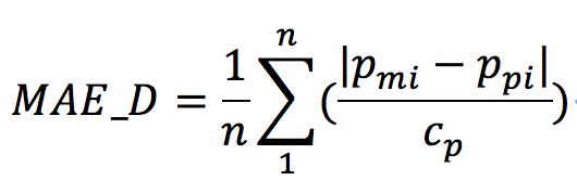
其中,MAE_D 为每日的平均绝对偏差,n为当天实际功率的值大于等于装机容量3%(即实际功率值大于等于Cp0.03)的测量样本的数量;Pmi为实际功率;Ppi为预测功率;Cp为装机容量。十个电站的装机功率依次为:20、30、10、20、21、10、40、30、50、20(单位MW)。
-
每月的绝对平均偏差的平均值计算方法如下:
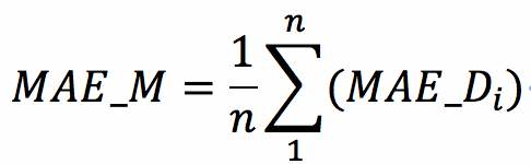
MAE_M为每月的绝对平均偏差,n为当月天数,MAE_Di为第i天的日平均绝对偏差。
这是本人第一次做的比较大的项目,由于是新手,可能很多方面做得不是很好。这里分享一下个人的经验和整个流程,排名不是很高,主要是提供一下思路,将之前学的知识应用到该项目中。
一、数据清洗
-
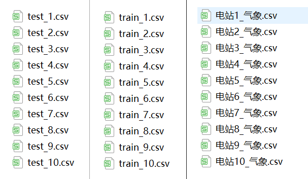
这里有3个文件夹,train文件夹存放训练数据,test文件夹存放测试数据,气象数据文件夹存放训练数据的气象数据。每个文件夹10个文件,对应10个不同的电场,如图1所示:
注意,训练数据集中有实际辐照度这个特征,而测试集中没有,且不能将实际辐照度作为特征来训练。所以有两种思路,一种是将实际辐照度作为标签来预测,通过预测得到的标签作为测试数据集的特征来进行训练;另一种是不考虑实际辐照度,由于实际辐照度和实际功率相关性太大,会降低其他气象数据的作用。这里我就不考虑实际辐照度这个特征了。
-
观察数据,查看数据包含哪些内容,查看训练数据集是否有缺失值,判断是否有缺失值后,若存在缺失值,可将其删除。
df.describe()  # 查看数据描述
df.head()    # 查看数据内容
df.isnull().any()    # 查看是否有缺失值
运行结果如图2、图3、图4所示:
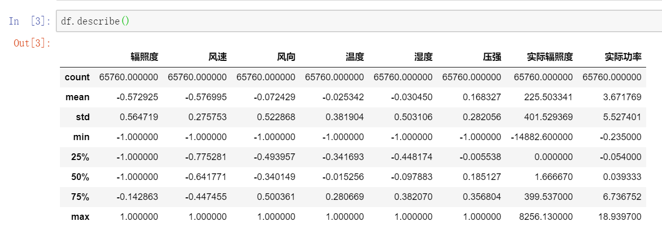
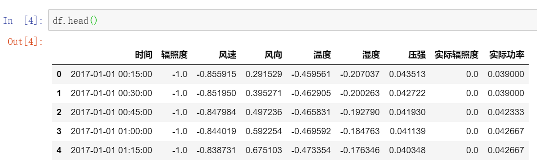
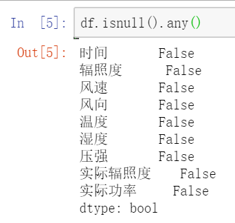
从图2中可以看出数据的整体描述;从图3可以看出特征有时间、辐照度、风速、风向、温度、湿度、压强、实际辐照度,要预测的是实际功率,而测试集中则不包含实际辐照度和实际功率;从图4可以看出数据不存在缺失值,不需要关注。
-
然后对数据进行可视化操作,主要分析辐照度、实际辐照度和实际功率的异常值。因为可能会出现晚上电场也在发电的情况,或者白天电场不工作的情况。考虑到每个电场的情况会不同,所以将每个电场单独进行分析,这里拿第1个电场进行全面的分析,参考代码:
"""
函数说明:数据可视化
Parameters:
	real_rad  - 实际辐照度
	real_power - 实际功率
	num - 电场编号
Returns:
	None
"""

def dataPlot(rad, real_rad, real_power, num):
    plt.figure(figsize=(12, 5))
    plt.title('第' + str(num+1) + '个训练场数据')
    plt.plot(rad.index, rad.values, label='辐照度', color='blue')
    plt.plot(real_rad.index, real_rad.values, label='实际辐照度', color='red')
    plt.plot(real_power.index, real_power.values, label='实际功率', color='green')
    plt.legend()
    plt.show()
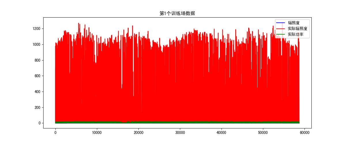
- 第一个电场如图5所示:
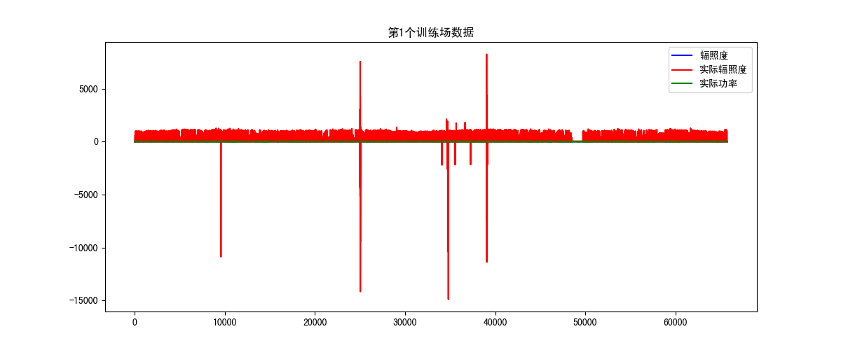
从图5可以看出实际辐照度存在负数和偏差大的值,还有一小段缺失值,这里可以通过左下角的图标放大来看。本人用的是Pycharm,需要设置'File'下的'Setting',找到'Tools'下的'Python Scientific',将'Show plots in tool winsow'的钩给去掉。放大后的图像如图6所示:
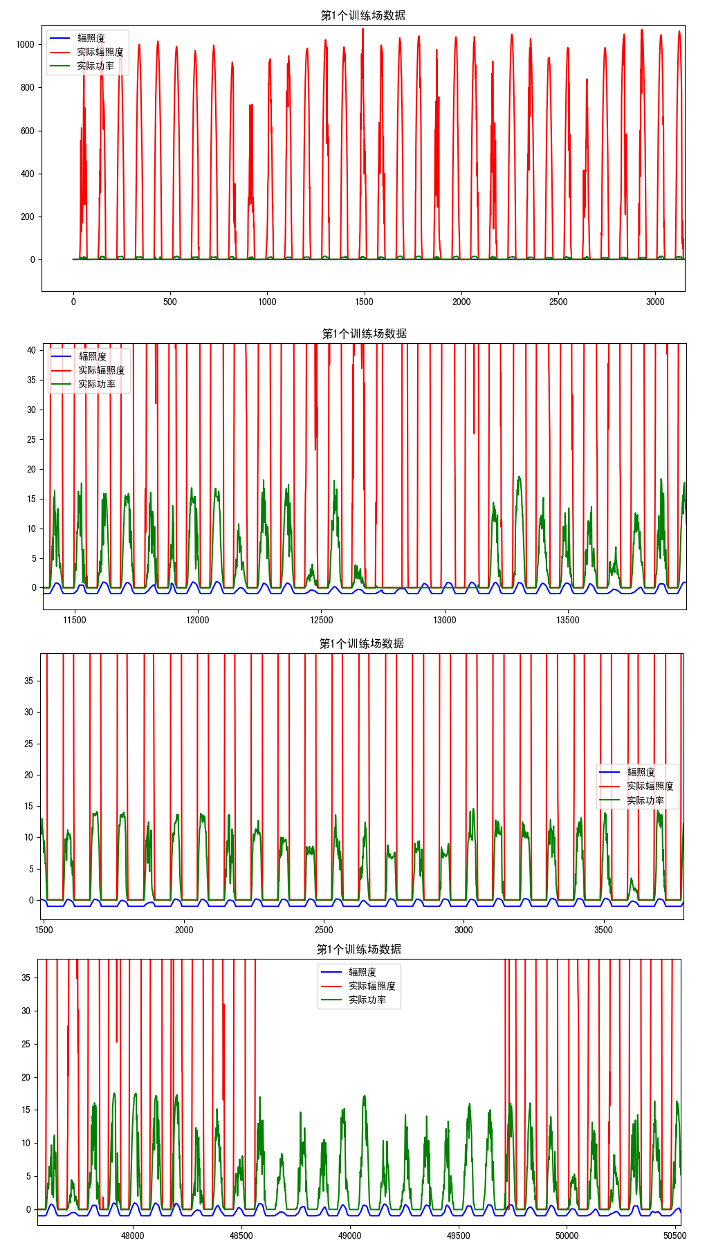
从图6我们可以粗略观察到三个数据的分布情况以及异常值,这里可以进一步放大,正常情况下实际辐照度大于实际功率,实际功率大于辐照度,否则就是异常值。通过观察异常数据并确定异常值出现的情况,建立异常值的索引,并将其删除,参考代码:
"""
函数说明:处理训练集1
Parameters:
	df - 训练数据集
Returns:
	df_new - 返回处理后的训练数据集
"""


def processDataset_1(df):
    # 实际辐照度大于等于0且小于1500
    df = df[(df['实际辐照度'].values >= 0) & (df['实际辐照度'].values < 1500)]
    # 实际辐照度大于实际功率
    df = df[df['实际辐照度'].values >= df['实际功率'].values]
    # 实际功率大于辐照度
    df = df[df['实际功率'].values > df['辐照度']]
    # 获取实际辐照度为48的索引
    drop_index = df[df['实际辐照度'].values == 48].index
    # 根据索引删除异常值
    df.drop(index=list(drop_index), inplace=True)
    # 重新建立索引
    df_new = df.reset_index(drop=True)

    return df_new
在处理每个电场数据之前,记得使用describe()函数和isnull().any()观察值,再进行处理。经过预处理后的数据如图7所示,放大后也没有异常值。
按照上面的思路将剩余的9个训练场进行异常值处理,由于每个电场的情况不一样,都需要通过图像去分析,这里每个电场的处理都不一样。
- 时间格式转换,将时间转换成年月日时分,参考程序如下:
"""
函数说明:时间格式处理
Parameters:
	date - 时间数据
Returns:
	time_list - 返回处理后的时间数据,包含年月日时分
"""

def dateFormat(date):
    time_list = []
    dt_new = pd.to_datetime(date)
    t = time.strptime(str(dt_new), '%Y-%m-%d %H:%M:%S')
    time_list.append(t.tm_year)
    time_list.append(t.tm_mon)
    time_list.append(t.tm_mday)
    time_list.append(t.tm_hour)
    time_list.append(t.tm_min)
    return time_list

# 将时间提取出来,转化为列表形式
sample_date = dt['时间'].values.tolist()
date_list = []  # 初始化一个空列表

for i in sample_date:  # 遍历date列,并将其格式转换为年、月、日、时、分
    date_list.append(dateFormat(i))  # 向列表添加年、月、日、时、分

sample_time = pd.DataFrame(date_list)  # 将列表转换为DataFrame
sample_time.columns = ['年', '月', '日', '时', '分']  # 给DataFrame添加列名

df = dt.reset_index(drop=True)  # 重新建立索引
df_new = pd.concat([sample_time, df], axis=1)  # 连接两个DataFrame
df_new.drop(columns=['时间'], inplace=True)  # 删除时间列

for i in sample_time.columns:  # 将时间数据类型转换为int32
    df_new[i] = df_new[i].astype('int32')
二、特征处理
接下来最主要的部分就是特征的处理了,一个模型的好坏主要取决于数据和特征的选择。数据和特征决定了机器学习的上限,而模型和算法是尽量接近这个上限,所以,特征是很重要的。
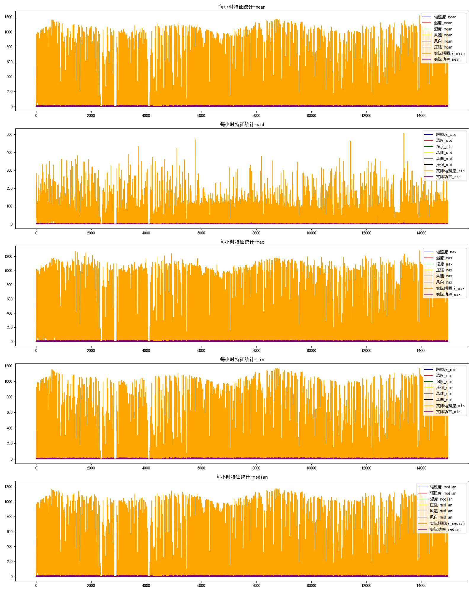
- 统计特征分析,这里将特征按照小时进行统计,分别计算每小时各项特征的均值、最值、标准差和中值,参考程序如下:
"""
函数说明:每小时的数据统计
Parameters:
	dt - 数据集
Returns:
    hourly_data - 返回统计后每小时的数据
"""


def statHourlydata(dt):
    drop_columns = dt.columns
    columns_date = ['年', '月', '日', '时']
    columns_old = ['辐照度', '风速', '风向', '温度', '湿度', '压强', '实际辐照度', '实际功率']

    # 统计均值
    hour_mean = dt.groupby(columns_date, as_index=False).mean()
    # 统计方差
    hour_std = dt.groupby(columns_date, as_index=False).std()
    # 统计中值
    hour_median = dt.groupby(columns_date, as_index=False).median()
    # 统计最值
    hour_max = dt.groupby(columns_date, as_index=False).max()
    hour_min = dt.groupby(columns_date, as_index=False).min()

    for i in columns_old:
        hour_mean[i + '_mean'] = hour_mean[i]
        hour_std[i + '_std'] = hour_std[i]
        hour_median[i + '_median'] = hour_median[i]
        hour_max[i + '_max'] = hour_max[i]
        hour_min[i + '_min'] = hour_min[i]
    hour_mean.drop(columns=drop_columns, inplace=True)
    hour_std.drop(columns=drop_columns, inplace=True)
    hour_median.drop(columns=drop_columns, inplace=True)
    hour_max.drop(columns=drop_columns, inplace=True)
    hour_min.drop(columns=drop_columns, inplace=True)

    frames = [hour_mean, hour_std, hour_median, hour_max, hour_min]
    hourly_data = pd.concat(frames, axis=1)
    return hourly_data


"""
函数说明:统计特征可视化
Parameters:
	df  - 数据集
Returns:
	None
"""

def statDataplot(df):
    fig = plt.figure(figsize=(16, 20))

    ax1 = fig.add_subplot(5, 1, 1)
    ax1.set_title('每小时特征统计-mean')
    ax1.plot(df['辐照度_mean'].values, label='辐照度_mean', color='blue')
    ax1.plot(df['温度_mean'].values, label='温度_mean', color='red')
    ax1.plot(df['湿度_mean'].values, label='湿度_mean', color='green')
    ax1.plot(df['风速_mean'].values, label='风速_mean', color='yellow')
    ax1.plot(df['风向_mean'].values, label='风向_mean', color='gray')
    ax1.plot(df['压强_mean'].values, label='压强_mean', color='black')
    ax1.plot(df['实际辐照度_mean'].values, label='实际辐照度_mean', color='orange')
    ax1.plot(df['实际功率_mean'].values, label='实际功率_mean', color='purple')
    ax1.legend()

    ax2 = fig.add_subplot(5, 1, 2)
    ax2.set_title('每小时特征统计-std')
    ax2.plot(df['辐照度_std'].values, label='辐照度_std', color='blue')
    ax2.plot(df['温度_std'].values, label='温度_std', color='red')
    ax2.plot(df['湿度_std'].values, label='湿度_std', color='green')
    ax2.plot(df['风速_std'].values, label='风速_std', color='yellow')
    ax2.plot(df['风向_std'].values, label='风向_std', color='gray')
    ax2.plot(df['压强_std'].values, label='压强_std', color='black')
    ax2.plot(df['实际辐照度_std'].values, label='实际辐照度_std', color='orange')
    ax2.plot(df['实际功率_std'].values, label='实际功率_std', color='purple')
    ax2.legend()

    ax3 = fig.add_subplot(5, 1, 3)
    ax3.set_title('每小时特征统计-max')
    ax3.plot(df['辐照度_max'].values, label='辐照度_max', color='blue')
    ax3.plot(df['温度_max'].values, label='温度_max', color='red')
    ax3.plot(df['湿度_max'].values, label='湿度_max', color='green')
    ax3.plot(df['压强_max'].values, label='压强_max', color='yellow')
    ax3.plot(df['风速_max'].values, label='风速_max', color='gray')
    ax3.plot(df['风向_max'].values, label='风向_max', color='black')
    ax3.plot(df['实际辐照度_max'].values, label='实际辐照度_max', color='orange')
    ax3.plot(df['实际功率_max'].values, label='实际功率_max', color='purple')
    ax3.legend()

    ax4 = fig.add_subplot(5, 1, 4)
    ax4.set_title('每小时特征统计-min')
    ax4.plot(df['辐照度_min'].values, label='辐照度_min', color='blue')
    ax4.plot(df['温度_min'].values, label='温度_min', color='red')
    ax4.plot(df['湿度_min'].values, label='湿度_min', color='green')
    ax4.plot(df['压强_min'].values, label='压强_min', color='yellow')
    ax4.plot(df['风速_min'].values, label='风速_min', color='gray')
    ax4.plot(df['风向_min'].values, label='风向_min', color='black')
    ax4.plot(df['实际辐照度_min'].values, label='实际辐照度_min', color='orange')
    ax4.plot(df['实际功率_min'].values, label='实际功率_min', color='purple')
    ax4.legend()

    ax5 = fig.add_subplot(5, 1, 5)
    ax5.set_title('每小时特征统计-median')
    ax5.plot(df['辐照度_median'].values, label='辐照度_median', color='blue')
    ax5.plot(df['温度_median'].values, label='辐照度_median', color='red')
    ax5.plot(df['湿度_median'].values, label='湿度_median', color='green')
    ax5.plot(df['压强_median'].values, label='压强_median', color='yellow')
    ax5.plot(df['风速_median'].values, label='风速_median', color='gray')
    ax5.plot(df['风向_median'].values, label='风向_median', color='black')
    ax5.plot(df['实际辐照度_median'].values, label='实际辐照度_median', color='orange')
    ax5.plot(df['实际功率_median'].values, label='实际功率_median', color='purple')
    ax5.legend()

    plt.show()
运行结果如图8所示:
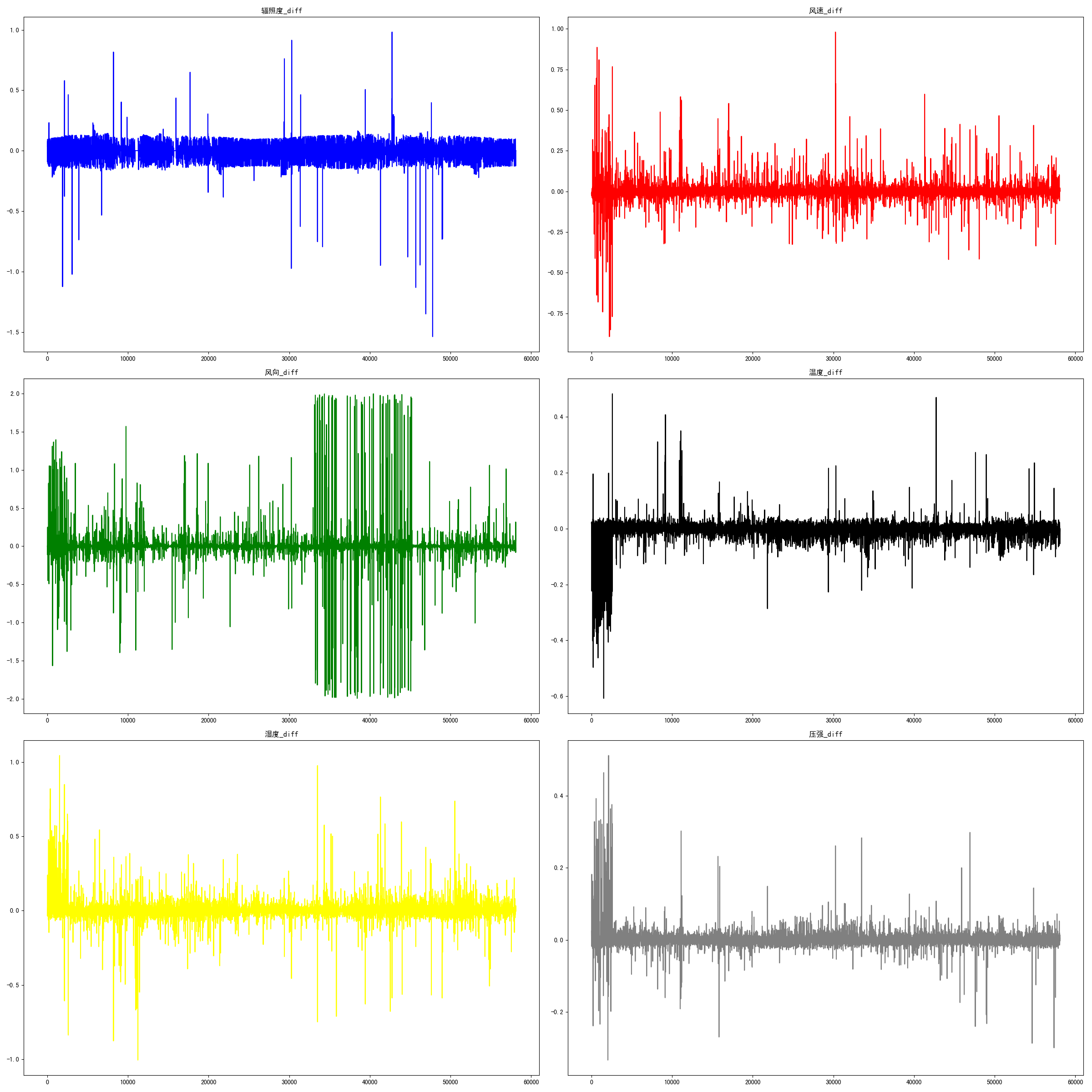
-
特征差分处理
这里主要的6个特征是辐照度、温度、湿度、风速、风向和压强,先对这6个特征进行差分处理,获取他们的差分特征,然后对其实行可视化操作,参考程序如下:
# 获取差分特征
df_new['辐照度_diff'] = df_new['辐照度'].diff()
df_new['风速_diff'] = df_new['风速'].diff()
df_new['风向_diff'] = df_new['风向'].diff()
df_new['温度_diff'] = df_new['温度'].diff()
df_new['湿度_diff'] = df_new['湿度'].diff()
df_new['压强_diff'] = df_new['压强'].diff()


"""
函数说明:差分数据可视化
Parameters:
   df  - 数据集
Returns:
   None
"""

def diffDataplot(df):
   fig = plt.figure(figsize=(24, 24))
   ax1 = fig.add_subplot(3, 2, 1)
   ax1.set_title('辐照度_diff')
   ax1.plot(df['辐照度_diff'].values, label='辐照度_diff', color='blue')

   ax2 = fig.add_subplot(3, 2, 2)
   ax2.set_title('风速_diff')
   ax2.plot(df['风速_diff'].values, label='风速_diff', color='red')

   ax3 = fig.add_subplot(3, 2, 3)
   ax3.set_title('风向_diff')
   ax3.plot(df['风向_diff'].values, label='风向_diff', color='green')

   ax4 = fig.add_subplot(3, 2, 4)
   ax4.set_title('温度_diff')
   ax4.plot(df['温度_diff'].values, label='温度_diff', color='black')

   ax5 = fig.add_subplot(3, 2, 5)
   ax5.set_title('湿度_diff')
   ax5.plot(df['湿度_diff'].values, label='湿度_diff', color='yellow')

   ax6 = fig.add_subplot(3, 2, 6)
   ax6.set_title('压强_diff')
   ax6.plot(df['压强_diff'].values, label='压强_diff', color='gray')
   plt.show()
可视化结果如图9所示:
- 接下来对时间进行处理,先将月份转划分为季节,参考程序如下:
"""
函数说明:将月份通过划分为四个季节
Parameters:
	dt_month - 月
Returns:
	df_season - 返回的季节,[1,2,3,4]对应春夏秋冬
"""

def divideSeason(dt_month):
    df_season = []
    for i in dt_month:
        if i == 1 or i == 2 or i == 12:
            df_season.append(4)
        elif i == 3 or i == 4 or i == 5:
            df_season.append(1)
        elif i == 6 or i == 7 or i == 8:
            df_season.append(2)
        else:
            df_season.append(3)
    return df_season
- 接下来的一些特征涉及到了天文学和地理学知识。通过查阅资料,了解到了一个比较重要的特征—太阳高度角,但是太阳高度角的计算公式比较复杂,所以分成了几步来计算。
- 1.先计算 时角:时角在正午最低,为0°,上午6点为-90°,下午为90°,在此时间段之外则将时角设为-90°。所以每小时时角变化15°,每15分钟则变化3.75°。所以,这里将'时'和'分'这两个特征进行处理,参考程序如下:
"""
函数说明:时角计算
Parameters:
	dt_hour - 时
	dt_min  - 分
Returns:
	time_angle - 返回当地的时角
"""

def divideHourlyAngle(dt_hour, dt_min):
    length = len(dt_hour)
    dt_hour = dt_hour.values
    dt_min = dt_min.values
    hour_angle = np.zeros((length,))
    pi = np.pi
    for i in range(length):
        if dt_hour[i] == 6:
            hour_angle[i] = -pi
        elif dt_hour[i] == 7:
            hour_angle[i] = -5 * pi / 6
        elif dt_hour[i] == 8:
            hour_angle[i] = -2 * pi / 3
        elif dt_hour[i] == 9:
            hour_angle[i] = -pi / 2
        elif dt_hour[i] == 10:
            hour_angle[i] = -pi / 3
        elif dt_hour[i] == 11:
            hour_angle[i] = -pi / 6
        elif dt_hour[i] == 12:
            hour_angle[i] = 0
        elif dt_hour[i] == 13:
            hour_angle[i] = pi / 6
        elif dt_hour[i] == 14:
            hour_angle[i] = pi / 3
        elif dt_hour[i] == 15:
            hour_angle[i] = pi / 2
        elif dt_hour[i] == 16:
            hour_angle[i] = 2 * pi / 3
        elif dt_hour[i] == 17:
            hour_angle[i] = 5 * pi / 6
        elif dt_hour[i] == 18:
            hour_angle[i] = pi
        elif dt_hour[i] >= 0 and dt_hour[i] < 6:
            hour_angle[i] = -pi
        else:
            hour_angle[i] = pi

    min_angle = np.zeros((length,))
    for i in range(length):
        if dt_hour[i] >= 6 and dt_hour[i] < 18 and dt_min[i] == 15:
            min_angle[i] = 3.75 * pi / 180
        elif dt_hour[i] >= 6 and dt_hour[i] < 18 and dt_min[i] == 30:
            min_angle[i] = 7.5 * pi / 180
        elif dt_hour[i] >= 6 and dt_hour[i] < 18 and dt_min[i] == 45:
            min_angle[i] = 11.25 * pi / 180
        else:
            min_angle[i] = 0

    time_angle = hour_angle + min_angle
    return time_angle
- 2.计算积日公式:积日,又称 年积日。公式涉及到了年月日这几个特征,参考程序如下:
"""
函数说明:积日公式
Parameters:
	year - 年
	month  - 月
	day - 日
Returns:
	result - 积日
"""

def calculateAccumulate(year, month, day):
    y = int(year)
    m = int(month)
    d = int(day)
    if y % 4 == 0 and y % 100 != 0 or y % 400 == 0:
        leap = 1
    else:
        leap = 0
    Accumulate = (0, 31, leap + 59, leap + 90, leap + 120, leap + 151, leap + 181,
                  leap + 212, leap + 243, leap + 273, leap + 304, leap + 334)
    result = Accumulate[m - 1] + d
    return result
- 3.赤纬算法,参考程序如下:
"""
"""
函数说明:赤纬算法
Parameters:
	year - 年
	month  - 月
	day - 日
Returns:
	direct_latitude - 返回太阳直射的纬度
"""


def calcutlateDeclination(year, month, day):
    length = len(year)
    year = year.values
    month = month.values
    day = day.values
    ED = np.zeros((length,))  # 赤纬角度
    for i in range(length):
        N = calculateAccumulate(year[i], month[i], day[i])
        N0 = 79.6764 + 0.2422 * (year[i] - 1985) - int((year[i] - 1985) / 4)
        theta = 2 * (np.pi) * (N - N0) / 365.2422
        delta = 0.3723 + 23.2567 * np.sin(theta) + 0.1149 * np.sin(2 * theta) - 0.1712 * np.sin(3 * theta) - \
                0.758 * np.cos(theta) + 0.3656 * np.cos(2 * theta) + 0.0201 * np.cos(3 * theta)
        ED[i] = abs(delta)
    direct_latitude = ED * np.pi / 180
    return direct_latitude
- 4.太阳高度角计算,参考程序如下:
"""
"""
函数说明:计算太阳高度角
Parameters:
	dt_time_angle - 太阳仰角
	dt_direct_latitude  - 太阳直射纬度
Returns:
	high_angle - 返回太阳的高度角
"""


def calculateSunAngle(dt_time_angle, dt_direct_latitude):
    length = len(dt_time_angle)
    direct_latitude = dt_direct_latitude.values
    elevate_angle = dt_time_angle.values
    high_angle = np.zeros((length,))
    phi = np.pi / 10
    for i in range(length):
        high_angle[i] = np.sin(phi) * np.sin(direct_latitude[i]) + np.cos(phi) * np.cos(direct_latitude[i]) * \
                        np.cos(elevate_angle[i])
    return high_angle
- 接下来进行特征组合,前面新添加了一些特征,将新旧特征进行交叉组合,得到新的组合特征,参考程序如下:
# 添加新特征
    df_new['温度_exp'] = np.exp(df_new['温度'])
    df_new['湿度_exp'] = np.exp(df_new['湿度'])
    df_new['压强_exp'] = np.exp(df_new['压强'])
    df_new['风速_exp'] = np.exp(df_new['风速'])
    df_new['时角_cos'] = np.cos(df_new['时角'])
    df_new['高度角_cos'] = np.cos(df_new['高度角'])
    df_new['直射纬度_cos'] = np.cos(df_new['直射纬度'])

    # 组合新特征
    df_new['时角_高度角'] = np.multiply(df_new['时角'], df_new['高度角'])
    df_new['直射纬度_时角'] = np.multiply(df_new['直射纬度'], df_new['时角'])
    df_new['直射纬度_高度角'] = np.multiply(df_new['直射纬度'], df_new['高度角'])
    df_new['温度_湿度_exp'] = np.multiply(df_new['温度_exp'], df_new['湿度_exp'])
    df_new['温度_湿度'] = np.multiply(df_new['温度'], df_new['湿度'])
    df_new['湿度_压强'] = np.multiply(df_new['湿度'], df_new['压强'])
    df_new['温度_压强'] = np.multiply(df_new['温度'], df_new['压强'])
    df_new['湿度_风速'] = np.multiply(df_new['湿度'], df_new['风速'])
    df_new['温度_风速'] = np.multiply(df_new['温度'], df_new['风速'])
- 这时,我们发现风向这个特征没有处理,考虑到风向不是一个连续值,所以需要对风向进行离散化处理,这里使用了KMeans算法和肘部法则,参考程序如下:
# 风向聚类离散化
data = df_new['风向'].values.reshape(-1, 1)
clf = KMeans(n_clusters=12).fit(data)
df_new['风向_离散'] = (clf.labels_) + 1
- 对季节和分这个特征进行one-hot处理,参考程序如下:
"""
函数说明:对季节和分进行one-hot处理
Parameters:
	dt - 数据集
Returns:
	dt - one-hot处理后的数据集
"""


def oneHot(dt):
    length = len(dt)
    dt_season = dt['季节'].values
    dt_min = dt['分'].values
    # 对季节进行one-hot处理
    season_1 = np.zeros((length,))
    season_2 = np.zeros((length,))
    season_3 = np.zeros((length,))
    season_4 = np.zeros((length,))
    for i in range(length):
        if dt_season[i] == 1:
            season_1[i] = 1
            season_2[i] = 0
            season_3[i] = 0
            season_4[i] = 0
        elif dt_season[i] == 2:
            season_1[i] = 0
            season_2[i] = 1
            season_3[i] = 0
            season_4[i] = 0
        elif dt_season[i] == 3:
            season_1[i] = 0
            season_2[i] = 0
            season_3[i] = 1
            season_4[i] = 0
        else:
            season_1[i] = 0
            season_2[i] = 0
            season_3[i] = 0
            season_4[i] = 1
    # 对分进行one-hot处理
    min_1 = np.zeros((length,))
    min_2 = np.zeros((length,))
    min_3 = np.zeros((length,))
    min_4 = np.zeros((length,))
    for i in range(length):
        if dt_min[i] == 15:
            min_1[i] = 1
            min_2[i] = 0
            min_3[i] = 0
            min_4[i] = 0
        elif dt_min[i] == 30:
            min_1[i] = 0
            min_2[i] = 1
            min_3[i] = 0
            min_4[i] = 0
        elif dt_min[i] == 45:
            min_1[i] = 0
            min_2[i] = 0
            min_3[i] = 1
            min_4[i] = 0
        else:
            min_1[i] = 0
            min_2[i] = 0
            min_3[i] = 0
            min_4[i] = 1

    dt['春季'] = season_1
    dt['夏季'] = season_2
    dt['秋季'] = season_3
    dt['冬季'] = season_4
    dt['15分'] = min_1
    dt['30分'] = min_2
    dt['45分'] = min_3
    dt['60分'] = min_4
    dt.drop(columns=['年', '季节', '分'], inplace=True)
    return dt
至此,特征的处理基本完成。
三、建立模型并预测
前面将特征处理好之后,接下来进行特征选择和建模。
- 首先进行特征选择,前面经过特征处理产生了一大堆新的特征,所以需要对特征进行选择,获取比较重要的特征。可以通过feature_importance来过滤掉一些特征,参考程序如下:
"""
函数说明:特征选择
Parameters:
	df- 训练数据集
	i - 电场编号
Returns:
	feature_choice - 选择的特征
"""


def featureChoice(df, i):
    feature = df.drop(columns=['实际功率', '实际辐照度'])
    label = df['实际功率']

    model = LGBMRegressor(n_estimators=40, num_leaves=30, max_depth=5)
    model.fit(feature.values, label.values)

    df_features = pd.DataFrame({'column': feature.columns,
                                'importance': model.feature_importances_}).sort_values(by='importance')
    # 可视化,并将结果保存到本地
    plt.figure(figsize=(12, 12))
    plt.barh(range(len(df_features)), df_features['importance'], height=0.8, alpha=0.6)
    plt.yticks(range(len(df_features)), df_features['column'])
    plt.title("第" + str(i + 1) + "个电场的 feature importance")
    plt.savefig('feature/' + '电场_' + str(i + 1) + '.jpg')
    # plt.show()

    df_features = df_features[df_features['importance'] > 25]  # 选择分数大于25的特征
    feature_choice = df_features['column'].values.tolist()
    return feature_choice
第一个电场的特征选择可视化结果如图11所示:
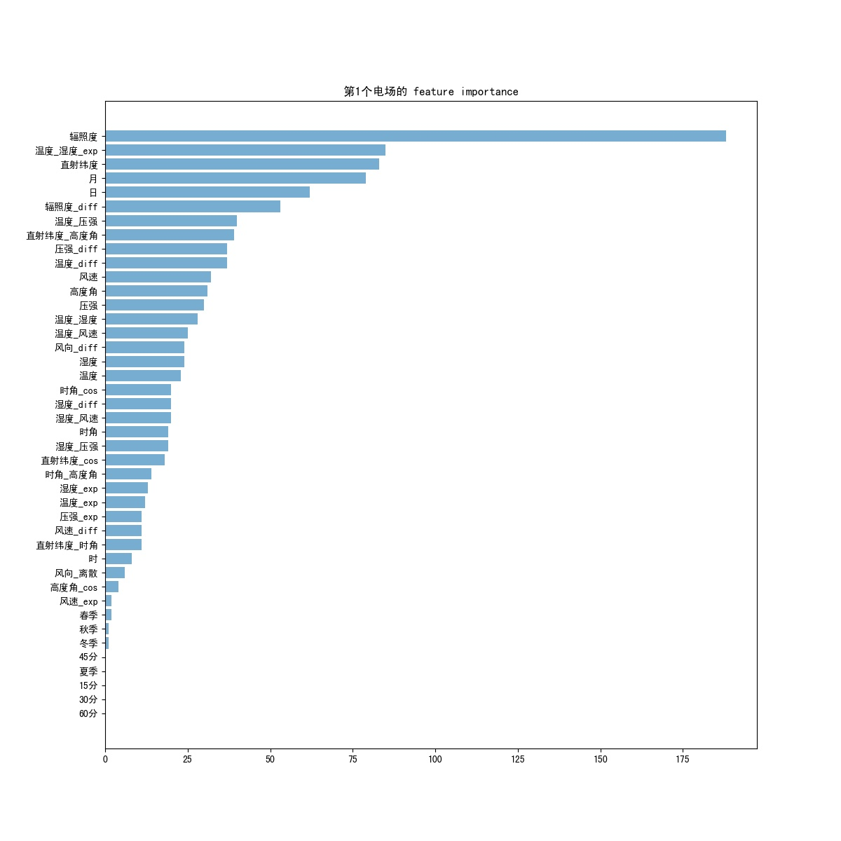
通过上述可视化结果自己设定阈值,选择合适的特征保留下来。
- 然后进行建模,这里使用LightGBM模型,在调参方面,使用了hyperopt 进行自动调参,参考程序如下:
"""
函数说明:自动调参
Parameters:
	df - 训练数据集
	p - 电场装机功率
Returns:
	best - 返回自动调参后的模型最优参数
"""

def trainParams(df, p):
    x = df.drop(columns=['实际功率']).values
    y = df['实际功率'].values
    print('划分数据集...')
    train_x, valid_x, train_y, valid_y = train_test_split(x, y, test_size=0.3, random_state=42)
    train = lgb.Dataset(train_x, train_y)
    valid = lgb.Dataset(valid_x, valid_y)

    # 自定义hyperopt的参数空间
    space = {"max_depth": hp.randint("max_depth", 10),
             "num_trees": hp.randint("num_trees", 100),
             'learning_rate': hp.randint('learning_rate', 20),
             "num_leaves": hp.randint("num_leaves", 20),
             "bagging_fraction": hp.randint("bagging_fraction", 6),
             "feature_fraction": hp.randint("feature_fraction", 6),
             "bagging_freq": hp.randint("bagging_freq", 3),
             "lambda_l1": hp.randint("lambda_l1", 10),
             "lambda_l2": hp.randint("lambda_l2", 10)
             }

    def argsDict_tranform(argsDict, isPrint=False):
        argsDict["max_depth"] = argsDict["max_depth"] + 10
        argsDict["num_trees"] = argsDict["num_trees"] * 10 + 100
        argsDict["learning_rate"] = argsDict["learning_rate"] * 0.005 + 0.01
        argsDict["num_leaves"] = argsDict["num_leaves"] * 2 + 10
        argsDict["bagging_fraction"] = argsDict["bagging_fraction"] * 0.1 + 0.4
        argsDict["feature_fraction"] = argsDict["feature_fraction"] * 0.1 + 0.4
        argsDict["bagging_freq"] = argsDict["bagging_freq"] + 3
        argsDict["lambda_l1"] = argsDict["lambda_l1"] * 0.1
        argsDict["lambda_l2"] = argsDict["lambda_l2"] * 0.01
        if isPrint:
            print(argsDict)
        else:
            pass
        return argsDict

    def lightgbm_factory(argsDict):
        argsDict = argsDict_tranform(argsDict)
        params = {'nthread': -1,  # 进程数
                  'max_depth': argsDict['max_depth'],  # 最大深度
                  'num_trees': argsDict['num_trees'],  # 树的数量
                  'learning_rate': argsDict['learning_rate'],  # 学习率
                  'num_leaves': argsDict['num_leaves'],  # 终点节点最小样本占比的和
                  'bagging_fraction': argsDict['bagging_fraction'],  # bagging采样数
                  'feature_fraction': argsDict['feature_fraction'],  # 样本列采样
                  'bagging_freq': argsDict["bagging_freq"],  # 每k次迭代执行bagging
                  'objective': 'regression',
                  'lambda_l1': argsDict["lambda_l1"],  # L1 正则化
                  'lambda_l2': argsDict["lambda_l2"],  # L2 正则化
                  'bagging_seed': 100  # 随机种子,light中默认为100
                  }
        params['metric'] = ['mae']

        model_lgb = lgb.train(params, train, num_boost_round=20000, valid_sets=[valid], early_stopping_rounds=100)
        return get_transformer_score(model_lgb)

    # 获取实际功率大于0.03*p的部分
    valid_y_new = valid_y[valid_y > 0.03 * p]
    valid_y_new_index = np.argwhere(valid_y > 0.03 * p)

    def get_transformer_score(transformer):
        model = transformer
        prediction = model.predict(valid_x, num_iteration=model.best_iteration)
        prediction_new = prediction[valid_y_new_index]
        return mean_absolute_error(valid_y_new, prediction_new)

    # 开始使用hyperopt进行自动调参
    algo = partial(tpe.suggest, n_startup_jobs=1)
    best = fmin(lightgbm_factory, space, algo=algo, max_evals=100, pass_expr_memo_ctrl=None)
    MAE = lightgbm_factory(best) / p
    print("The best of MAE is: %s" % MAE)

    # 返回MAE和最优参数
    return MAE, best
-
然后将上面的模型参数去预测测试集。
-
模型优化:将预测的结果进行线上检验,第一次线上的结果比线下的要差很多,出现了过拟合。可以增加正则化函数l1、l2,减少过拟合。
调参参考:
- For Faster Speed
Use bagging by setting
bagging_fractionandbagging_freq
Use feature sub-sampling by settingfeature_fraction
Use smallmax_bin
Usesave_binaryto speed up data loading in future learning Useparallel learning, refer to Parallel Learning Guide
- For Better Accuracy
Use large
max_bin(may be slower)
Use smalllearning_ratewith largenum_iterationsUse largenum_leaves(may cause over-fitting)
Use bigger training data
Trydart
- Deal with Over-fitting
Use small
max_bin
Use smallnum_leaves
Usemin_data_in_leafandmin_sum_hessian_in_leaf
Use bagging by setbagging_fractionandbagging_freq
Use feature sub-sampling by setfeature_fraction
Use bigger training data
Trylambda_l1, lambda_l2andmin_gain_to_splitfor regularization
Trymax_depthto avoid growing deep tree
四、总结:
-
1.数据清洗方面:
个人是对每一个电场都放大进行分析,这个过程比较耗时,但是异常值也清洗得比较干净。但是也会把一些正常数据给清洗掉,比如雨天、沙尘暴天气,辐射度正常,但是实际功率很低,这样的话可能会降低气象数据对模型的权重,而且也会降低模型的泛化能力。但是不放大分析的话,又有可能有许多噪声数据,模型将异常数据当做正常数据来分析,这样模型的泛化效果也会降低。所以,权衡利弊,个人还是选择放大进行数据清洗。
-
2.特征处理方面:这个过程是最麻烦的。
- 首先,时间格式要转换为年月日时分。在光伏发电中,时间是一个很重要的特征,季节不同、时间不同,发电量也不同。所以时间特征可以继续划分,比如白天和夜晚,按季节可分为四季,等等。
- 接下来是差分特征,这也是一个比较重要的特征,从第二行开始,求所有维度上本行与上一行的差,可以反映样本在各个特征上的变化。
- 统计特征,常见的有均值、方差、标准差、中位数等,可以有效标识出数据的特点,还有峰度和偏度等,我选择的是每小时辐照度、温度、湿度、风速、风向、压强的标准差,太多了就没有用,以后可以尝试。
- 然后是太阳高度角,这是我在查询资料时发现的一个比较厉害的特征,但是没有电场当地纬度,所以就设置了一个比较好算的值为当地纬度,其实可以将当地纬度作为一个变量,通过太阳高度角公式计算出和实际辐照度相关度最大时的纬度即为当地纬度。当中还涉及到时角、积日、赤纬算法等。
- 接下来是特征组合,寻找高维特征,将特征进行交叉组合,但是也有许多无用的组合,到后面再处理。
- 然后是离散化处理,风向是一个离散的数据,而在这里是连续的值,所以使用KMeans算法对其进行离散化处理。
- 接着对category数据进行one-hot处理,比如季节、风向。
-
3.特征选择,可以使用feature_importance来进行特征选择,将一些重要的特征保存下来。特征少了,机器会学不到,特征多了,又会影响模型的效果,所以阈值需要稍微调试一下。
-
4.建立模型并预测:
- 在建立模型的时候,选择一个合适的模型是很重要的,这里我选择了LightGBM,主要是会用,也符合这种场景,更多的可以选择神经网络。
- 首先是设定参数范围,不能太大,也不能太小,这个看经验了。第一次设定的时候参数给的太大,结果出现过拟合,后面通过减少了树的深度,增大学习率,对数据进行正则化来优化模型。
- 然后是调参,这是一个考验经验的步骤,初始参数不能乱给,这里我在网上查阅,找到了一个自动调参模块hyperopt,大大节省了时间。一开始是用RandomizedSearchCV,但是搜索结果有随机性,不一定是最优;然后试了试网格搜素GridSearchCV,这个方法是对每个参数进行组合,找到的结果是最好的,但是很耗时间和内存,不适合大范围调参。
- 这里我并没有使用模型融合这个大杀器,听说很有用。模型差异性可以通过特征多样性、参数多样性、模型多样性来做到。只有好而不同的模型,融合才是有意义的,因为不同的模型偏好不一样,犯错的样本也不一样,因而可以取长补短,提升效果。但是,只有单模做好了,多模融合才有用,所以我只用了单模,多模融合以后再用。这里给大家放模型融合的例子: 模型融合,大家可以参考一下。
学习数据分析也有一段时间了,过去都是拿着书上的代码照着敲,最多就是处理完异常值直接拿模型去预测数据,特征工程也没有做,模型参数也没有优化。通过这次竞赛也算是积累经验了,中间遇到过很多问题,都一一解决了。总体来看,个人在算法的理解上还不到位,对数据的了解也不够深,还需要多多努力有很多不足的地方,请大家指出。
