

逻辑回归(Logistic Regression)是一种用于解决二分类(0 or 1)问题的机器学习方法,可以用于估计某种事物的可能性。比如某用户购买某商品的可能性,某病人患有某种疾病的可能性,以及某广告被用户点击的可能性等。
本文的一个大致目录如下:
- 选取预测函数。
- 计算损失函数。
- 使用梯度下降计算损失函数最小值。
- 向量化。
- 基于梯度下降实现逻辑回归算法。
- 多项式特征。
- 多分类。
- 正则化。
预测函数
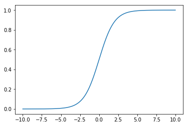
逻辑回归虽然带有回归二字,但实际上它是一种分类算法,可用于二分类问题(当然也可用于多分类问题下面章节会做介绍)。预测函数选择的是 Sigmoid 函数,函数表达式如下:
可以使用 Python 代码来绘制一下:
import numpy as np
import matplotlib.pyplot as plt

def sigmoid(t):
    return 1. / (1. + np.exp(-t))

x = np.linspace(-10, 10, 500)

plt.plot(x, sigmoid(x))
plt.show()
对于线性边界的情况,其表达形式为:
定义预测函数为:
表示为结果取 1 的概率,因此:
构造损失函数
损失函数的定义如下:
做一下转换:
梯度下降求解损失函数
求损失函数的最小值可以使用梯度下降法,其中 为学习步长:
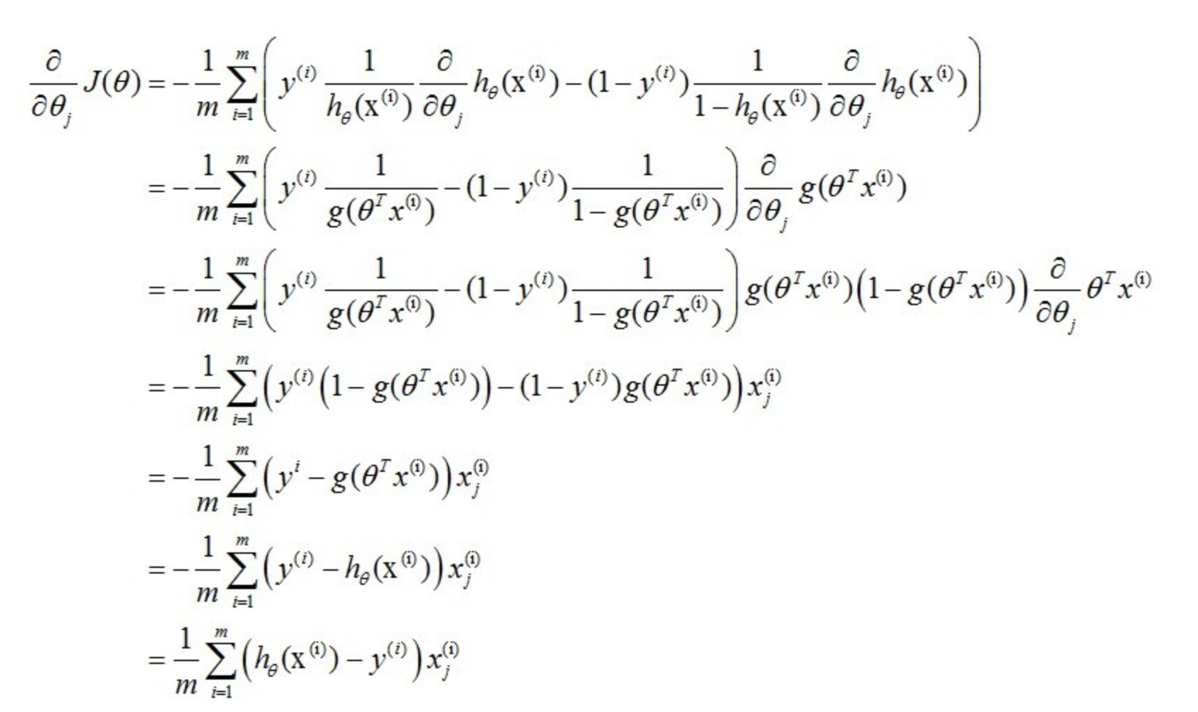
下面是求偏导之后的一个结果:
具体的一个求导过程如下:
所以:
因为 1/m 是一个常数, 也为一个常量,所以最终的一个表达式为:
向量化
向量化后最终的一个结果为:
具体推导一下-todo
Python 实现逻辑回归
下面是用 Python 代码实现的一个逻辑回归算法,对于优化损失函数使用的是梯度下降的方法。
def __init__(self):
    self.coef_ = None
    self.intercept_ = None
    self._theta = None

def _sigmoid(self, t):
    return 1. / (1. + np.exp(-t))

def fit(self, X_train, y_train, eta=0.01, n_iters=1e4):
    X_b = np.hstack([np.ones((len(X_train), 1)), X_train])
    initial_theta = np.zeros(X_b.shape[1])
    self._theta = gradient_descent(X_b, y_train, initial_theta, eta, n_iters)

    self.intercept_ = self._theta[0]
    self.coef_ = self._theta[1:]
    return self
梯度下降的实现代码如下:
def J(theta, X_b, y):
    y_hat = self._sigmoid(X_b.dot(theta))
    try:
        return - np.sum(y*np.log(y_hat) + (1-y)*np.log(1-y_hat)) / len(y)
    except:
        return float('inf')

def dJ(theta, X_b, y):
    return X_b.T.dot(self._sigmoid(X_b.dot(theta)) - y) / len(y)

def gradient_descent(X_b, y, initial_theta, eta, n_iters=1e4, epsilon=1e-8):
    theta = initial_theta
    cur_iter = 0

    while cur_iter < n_iters:
        gradient = dJ(theta, X_b, y)
        last_theta = theta
        theta = theta - eta * gradient
        if (abs(J(theta, X_b, y) - J(last_theta, X_b, y)) < epsilon):
            break

        cur_iter += 1

    return theta
预测方法和得分方法:
def predict(self, X_predict):
    assert self.intercept_ is not None and self.coef_ is not None, \
        "must fit before predict!"
    assert X_predict.shape[1] == len(self.coef_), \
        "the feature number of X_predict must be equal to X_train"

    X_b = np.hstack([np.ones((len(X_predict), 1)), X_predict])
    proba = self._sigmoid(X_b.dot(self._theta))
    return np.array(proba >= 0.5, dtype='int')

def score(self, X_test, y_test):
    y_predict = self.predict(X_test)
    assert len(y_true) == len(y_predict), \
               "the size of y_true must be equal to the size of y_predict"

    return np.sum(y_true == y_predict) / len(y_true)
多项式特征
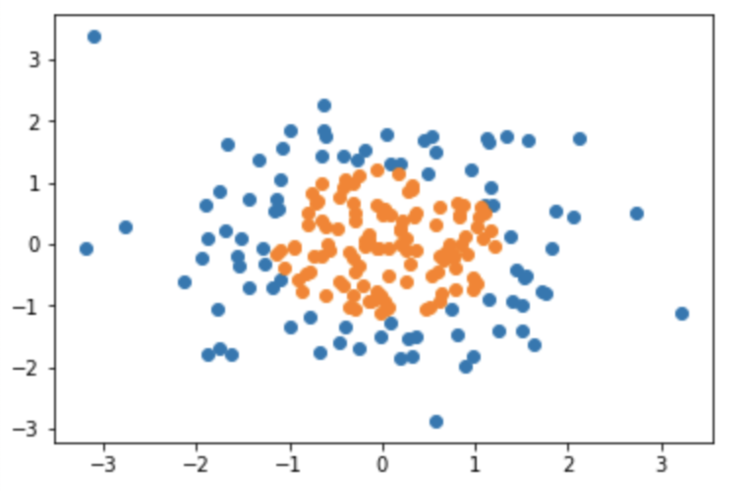
上述我们的假设,都是将决策边界看作是一条直线。很多时候样本点的分布是非线性的。我们可以引入多项式项,进而改变样本的分布状态。
首先我们模拟一个非线性分布的数据集:
import numpy as np
import matplotlib.pyplot as plt

np.random.seed(666)
X = np.random.normal(0, 1, size=(200, 2))
y = np.array(X[:,0]**2 + X[:,1]**2 < 1.5, dtype='int')

plt.scatter(X[y==0,0], X[y==0,1])
plt.scatter(X[y==1,0], X[y==1,1])
plt.show()
对于这样一个数据集,只能添加多项式来解决,代码如下:
from sklearn.pipeline import Pipeline
from sklearn.preprocessing import PolynomialFeatures
from sklearn.preprocessing import StandardScaler

def PolynomialLogisticRegression(degree):
    return Pipeline([
        # 给样本特征添加多形式项;
        ('poly', PolynomialFeatures(degree=degree)),
        # 数据归一化处理;
        ('std_scaler', StandardScaler()),
        ('log_reg', LogisticRegression())
    ])

poly_log_reg = PolynomialLogisticRegression(degree=2)
poly_log_reg.fit(X, y)

plot_decision_boundary(poly_log_reg, axis=[-4, 4, -4, 4])
plt.scatter(X[y==0,0], X[y==0,1])
plt.scatter(X[y==1,0], X[y==1,1])
plt.show()
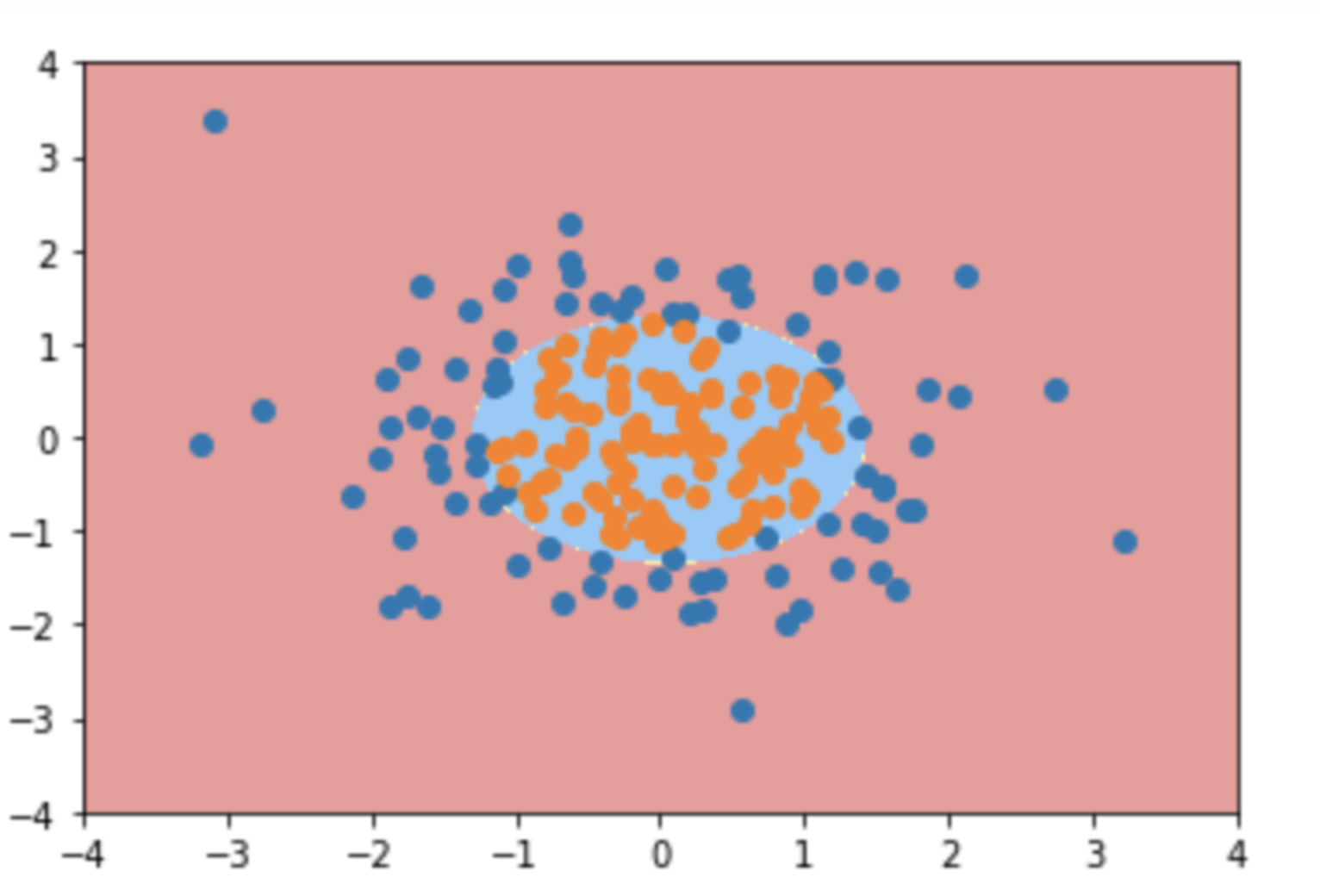
最终数据的决策边界如下:
def plot_decision_boundary(model, axis):
    x0, x1 = np.meshgrid(
        np.linspace(axis[0], axis[1], int((axis[1]-axis[0])*100)).reshape(-1,1),
        np.linspace(axis[2], axis[3], int((axis[3]-axis[2])*100)).reshape(-1,1)
    )
    X_new = np.c_[x0.ravel(), x1.ravel()]

    y_predict = model.predict(X_new)
    zz = y_predict.reshape(x0.shape)

    from matplotlib.colors import ListedColormap
    custom_cmap = ListedColormap(['#EF9A9A','#FFF59D','#90CAF9'])

    plt.contourf(x0, x1, zz, linewidth=5, cmap=custom_cmap)
多分类问题
上面我们提到逻辑回归只能解决二分类问题,处理多分类问题需要额外转换一下。通常有两种途径:
- OVR(One vs Rest),一对剩余的意思。
- OVO(One vs One),一对一的意思。
这两种方法不仅仅可以针对逻辑回归算法,对于所有二分类机器学习算法都可以使用此方法进行改造,将二分类问题转换成多分类问题。
OVR
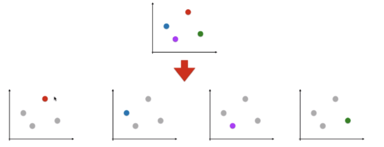
如上图所示,对 n 种类型的样本进行分类时,分别取某一类样本作为一类,将剩下 n-1 类样本看作是另外一类,这样就可以转换成 n 个二分类问题。最终可以得到 n 个算法模型(如上图所示,最终会有 4 个算法模型),将待预测的样本分别传入这 n 个模型中,所得概率最高的那个模型对应的样本类型为预测结果。
在 sklearn 中对于逻辑回归的多分类问题,默认采用的就是 ovo 的方式。同时 sklearn 也提供了一种通用的调用方式:
from sklearn.multiclass import OneVsRestClassifier
from sklearn.linear_model import LogisticRegression

log_reg = LogisticRegression()
ovr = OneVsRestClassifier(log_reg)
ovr.fit(X_train, y_train)
ovr.score(X_test, y_test)
OVO
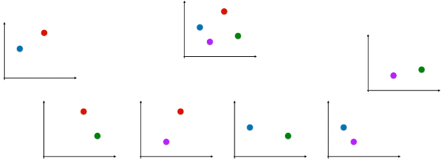
n 类样本中,每次挑选出两类样本,最终形成 种二分类情况,也就是
个算法模型,有
个预测结果,这些结果中种类最多的样本类型,就是最终的预测结果。
在 sklearn 逻辑回归的实现中,对于多分类默认使用的是 ovr,如果使用 ovo 的话需要指定一下 multi_class,同时 solver 参数也需要改一下(p.s: sklearn 中对于损失函数最有化不是采用上述我们描述的梯度下降):
import numpy as np
import matplotlib.pyplot as plt
from sklearn import datasets
from sklearn.model_selection import train_test_split
from sklearn.linear_model import LogisticRegression

iris = datasets.load_iris()

X = iris.data
y = iris.target

X_train, X_test, y_train, y_test = train_test_split(X, y, random_state=666)

log_reg2 = LogisticRegression(multi_class="multinomial", solver="newton-cg")
log_reg2.fit(X_train, y_train)
log_reg2.score(X_test, y_test)
from sklearn.multiclass import OneVsRestClassifier

ovr = OneVsRestClassifier(log_reg)
ovr.fit(X_train, y_train)
ovr.score(X_test, y_test)

from sklearn.multiclass import OneVsOneClassifier

ovo = OneVsOneClassifier(log_reg)
ovo.fit(X_train, y_train)
ovo.score(X_test, y_test)
正则化
通常正则化的表达形式如下:
可以转换一下,改变超参数位置。如果超参数 C 越大,原损失函数 的地位相对较重要。如果超参数非常小,正则项的地位相对较重要。如果想让正则项不重要,需要增大参数 C。sklearn 中一般都是采用的这样的表达方式。
sklearn 中的逻辑回归算法自动封装了模型的正则化的功能,只需要调整 C 和 penalty(正则项选择 或者
。
