

原文:Deep Learning From Scratch III: Training Criterion - deep ideas
翻译:孙一萌
- 第一章:计算图
- 第二章:感知机
- 第三章:训练标准
- 第四章:梯度下降与反向传播
- 第五章:多层感知机
- 第六章:TensorFlow
Training criterion
现在我们学会了用线性分类器将点分类,以及计算点属于某个特定分类的概率,只要我们给权矩阵 和偏置
一个合适的值。
那么自然我们就遇到一个问题:怎样给权矩阵 和偏置
一个合适的值。在红/蓝的例子中,我们就光观察了一下训练数据,然后靠猜得到一条线,把平面上的点完美地分割成了两部分。
但一般来说,我们不想亲手去找出一条分割线,我们希望的是,把训练点提供给计算机之后,它可以自己找到一条好的分割线。
那么我们怎么评价分割线是好是坏呢?
错分率(The misclassification rate)
理想情况下,我们希望找到一条错误尽可能少的分割线。我们不知道真实的数据生成分布 是什么样的,但是对于其中的每一个点 x 及其所属的每一个分类 c(x),我们都希望使感知机分类错误的概率最小。也就是最小化
错分率:
通常情况下,我们不知道真实的数据生成分布 的情况,所以计算出错分率的确切数值是不可能的。但是我们是有一组训练点的,这些训练点里包含 x 的值和它所属的分类。
在后文中,我们会用形如 的矩阵代指一组训练点,每一行代表一个训练点,矩阵列的数目等于训练点的维数,每一列代表一个维度。
除此以外,我们把真实正确的分类情况用矩阵 表示,如果第
个训练样本拥有分类
,那么
[math]$ c_{i,j} = 1 $[/math] 。相似地,我们也用一个矩阵 代表预期的分类情况,如果第
个训练样本的预测类别是
,那么
。
最后,我们用矩阵 来表示概率,其中
表示第
个训练样本属于类别
的概率。
通过训练数据,我们能找到一个样本错分率最低的分类器:
然而我们发现,要找到错分率最低的线性分类器非常困难:随着输入数据的维度的提高,计算复杂度呈指数级增长,找到这个线性分类器显得不切实际。
就算我们找到了错分率最低的分类器,它也可能通过把类别区分得更开,使得自己更具鲁棒性以应对未知数据,即便它这么做并不会降低样本错分率。
最大似然估计
替代方法是最大似然估计,在最大似然估计中,我们尝试寻找特定的参数值,来使得概率 最大化。
此处我们引入
被称为交叉熵损失。此处我们希望把
最小化。
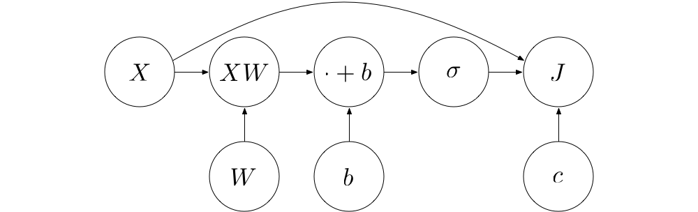
我们把 看成一个
Operation,那么它的输入就有:数据 、真实的分类情况
和预期概率
。
即 operation
的输出。
这样就可以计算出损失的真实数字:
建造一个用于计算  的
的 operation
要建造用于计算 的
operaion,我们可以把多个初级一些的 operation 结合起来。首先, 可以用矩阵运算
作如下表示:
从中我们可以发现,上述的“初级一些”的 operation 有如下几种:
-
log:矩阵或者向量的,对每个元素进行的对数(log)运算
-
⊙:两个矩阵之间,对每个元素进行的乘法运算
-
:矩阵所有列的总和
-
:矩阵所有行的总和
-
−:逐元素负运算
然后我们将它们分别实现一下。
1. log
对张量(tensor)的逐元素对数运算:
class Operation:
    """Represents a graph node that performs a computation.

    An `Operation` is a node in a `Graph` that takes zero or
    more objects as input, and produces zero or more objects
    as output.
    """

    def __init__(self, input_nodes=[]):
        """Construct Operation
        """
        self.input_nodes = input_nodes

        # Initialize list of consumers (i.e. nodes that receive this operation's output as input)
        self.consumers = []

        # Append this operation to the list of consumers of all input nodes
        for input_node in input_nodes:
            input_node.consumers.append(self)

        # Append this operation to the list of operations in the currently active default graph
        _default_graph.operations.append(self)

    def compute(self):
        """Computes the output of this operation.
        "" Must be implemented by the particular operation.
        """
        pass

class Graph:
    """Represents a computational graph
    """

    def __init__(self):
        """Construct Graph"""
        self.operations = []
        self.placeholders = []
        self.variables = []

    def as_default(self):
        global _default_graph
        _default_graph = self

class placeholder:
    """Represents a placeholder node that has to be provided with a value
       when computing the output of a computational graph
    """

    def __init__(self):
        """Construct placeholder
        """
        self.consumers = []

        # Append this placeholder to the list of placeholders in the currently active default graph
        _default_graph.placeholders.append(self)

class Variable:
    """Represents a variable (i.e. an intrinsic, changeable parameter of a computational graph).
    """

    def __init__(self, initial_value=None):
        """Construct Variable

        Args:
          initial_value: The initial value of this variable
        """
        self.value = initial_value
        self.consumers = []

        # Append this variable to the list of variables in the currently active default graph
        _default_graph.variables.append(self)

class add(Operation):
    """Returns x + y element-wise.
    """

    def __init__(self, x, y):
        """Construct add

        Args:
          x: First summand node
          y: Second summand node
        """
        super().__init__([x, y])

    def compute(self, x_value, y_value):
        """Compute the output of the add operation

        Args:
          x_value: First summand value
          y_value: Second summand value
        """
        return x_value + y_value

class matmul(Operation):
    """Multiplies matrix a by matrix b, producing a * b.
    """

    def __init__(self, a, b):
        """Construct matmul

        Args:
          a: First matrix
          b: Second matrix
        """
        super().__init__([a, b])

    def compute(self, a_value, b_value):
        """Compute the output of the matmul operation

        Args:
          a_value: First matrix value
          b_value: Second matrix value
        """
        return a_value.dot(b_value)
class Session:
    """Represents a particular execution of a computational graph.
    """

    def run(self, operation, feed_dict={}):
        """Computes the output of an operation

        Args:
          operation: The operation whose output we'd like to compute.
          feed_dict: A dictionary that maps placeholders to values for this session
        """

        # Perform a post-order traversal of the graph to bring the nodes into the right order
        nodes_postorder = traverse_postorder(operation)

        # Iterate all nodes to determine their value
        for node in nodes_postorder:

            if type(node) == placeholder:
                # Set the node value to the placeholder value from feed_dict
                node.output = feed_dict[node]
            elif type(node) == Variable:
                # Set the node value to the variable's value attribute
                node.output = node.value
            else:  # Operation
                # Get the input values for this operation from node_values
                node.inputs = [input_node.output for input_node in node.input_nodes]

                # Compute the output of this operation
                node.output = node.compute(*node.inputs)

            # Convert lists to numpy arrays
            if type(node.output) == list:
                node.output = np.array(node.output)

        # Return the requested node value
        return operation.output


def traverse_postorder(operation):
    """Performs a post-order traversal, returning a list of nodes
    in the order in which they have to be computed

    Args:
       operation: The operation to start traversal at
    """

    nodes_postorder = []

    def recurse(node):
        if isinstance(node, Operation):
            for input_node in node.input_nodes:
                recurse(input_node)
        nodes_postorder.append(node)

    recurse(operation)
    return nodes_postorder

class softmax(Operation):
    """返回 a 的 softmax 函数结果.
    """

    def __init__(self, a):
        """构造 softmax

        参数列表:
          a: 输入节点
        """
        super().__init__([a])

    def compute(self, a_value):
        """计算 softmax operation 的输出值

        参数列表:
          a_value: 输入值
        """
        return np.exp(a_value) / np.sum(np.exp(a_value), axis=1)[:, None]
class log(Operation):
    """ 对每一个元素进行对数运算
    """

    def __init__(self, x):
        """ 构造 log

        参数列表:
          x: 输入节点
        """
        super().__init__([x])

    def compute(self, x_value):
        """ 计算对数 operation 的输出

        参数列表:
          x_value: 输入值
        """
        return np.log(x_value)
2. 乘法 / ⊙
对两个同样形状的张量的逐元素乘法运算
class multiply(Operation):
    """ 对每一个元素,返回 x * y 的值
    """

    def __init__(self, x, y):
        """ 构造乘法

        参数列表:
          x: 第一个乘数的输入节点
          y: 第二个乘数的输入节点
        """
        super().__init__([x, y])

    def compute(self, x_value, y_value):
        """ 计算乘法 operation 的输出

        Args:
          x_value: 第一个乘数的值
          y_value: 第二个乘数的值
        """
        return x_value * y_value
3. reduce_sum
为了在单个 operation 里计算多种总和(比如所有行的总和、所有列的总和等等),我们指定一个值 axis,如果 axis = 0 就表示计算行的总和,axis = 1 表示计算列的总和,等等等等。Numpy 就是这样实现的。
class reduce_sum(Operation):
    """ 计算张量中元素延某一或某些维度的总和
    """

    def __init__(self, A, axis=None):
        """ 构造 reduce_sum

        参数列表:
          A: 要进行 reduce 运算的张量
          axis: 需要 reduce 的维度,如果 `None`(即缺省值),则延所有维度 reduce
        """
        super().__init__([A])
        self.axis = axis

    def compute(self, A_value):
        """ 计算 reduce_sum operation 的输出值

        参数列表:
          A_value: 输入的张量值
        """
        return np.sum(A_value, self.axis)
4. 负运算
对张量的每个元素进行负运算:
class negative(Operation):
    """ 逐元素计算负数
    """

    def __init__(self, x):
        """ 构造负运算

        参数列表:
          x: 输入节点
        """
        super().__init__([x])

    def compute(self, x_value):
        """ 计算负运算 operation 的输出

        参数列表:
          x_value: 输入值
        """
        return -x_value
5. 结合这些 operation
用上述这些 operation,我们现在可以把 J 的运算写成如下形式:
J = negative(reduce_sum(reduce_sum(multiply(c, log(p)), axis=1)))
### 举例 现在我们来计算一下红/蓝 perceptron 的损失
import numpy as np
red_points = np.random.randn(50, 2) - 2*np.ones((50, 2))
blue_points = np.random.randn(50, 2) + 2*np.ones((50, 2))

# 创建一个新的 graph
Graph().as_default()

X = placeholder()
c = placeholder()

W = Variable([
    [1, -1],
    [1, -1]
])
b = Variable([0, 0])
p = softmax(add(matmul(X, W), b))

# 交叉熵损失
J = negative(reduce_sum(reduce_sum(multiply(c, log(p)), axis=1)))

session = Session()
print(session.run(J, {
    X: np.concatenate((blue_points, red_points)),
    c:
        [[1, 0]] * len(blue_points)
        + [[0, 1]] * len(red_points)

}))
如果你有什么疑问,尽管在评论区提出。
