Deep Learning #3: More on CNNs & Handling Overfitting

What are convolutions, max pooling and dropout?

This post is part of a series on deep learning. Check-out part 1 and part 2.

Welcome to the third entry in this series on deep learning! This week I will explore some more parts of the Convolutional Neural Network (CNN) and will also discuss how to deal with underfitting and overfitting.

Convolutions

So what exactly is a convolution? As you might remember from my previous blog entries we basically take a small filter and slide this filter over the whole image. Next, the pixel values of the image are multiplied with the pixel values in the filter. The beauty in using deep learning is that we do not have to think about how these filters should look. Through Stochastic Gradient Descent (SGD) the network is able to learn the optimal filters. The filters are initialized at random and are location-invariant. This means that they can find something everywhere in the image. At the same time the model also learns where in the image it has found this thing.

Zero padding is a helpful tool when applying this filters. All this does, is at extra borders of zero pixels around the image. This allows us to also capture the edges of the images when sliding the filter over the image. You might wonder what size the filters should be. Research has shown that smaller filters generally perform better. In this case we use filters of size 3x3.

When we slide these filters over our image we basically create another image. Therefore, if our original image was 30x30 the output of a convolutional layer with 12 filters will be 30x30x12. Now we have a tensor, which basically is a matrix with over 2 dimensions. Now you also know where the name TensorFlow comes from.

After each convolutional layer (or multiple) we typically have a max pooling layer. This layer simply reduces the amount of pixels in the image. For example, we can take a square of our image and replace this with only the highest value on the square.

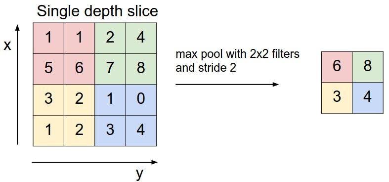
Because of Max Poling our filters can explore bigger parts of the image. Additionally, because of the loss in pixels we typically increase the number of filters after used max pooling.

In theory every model architecture will work and should be able to provide a good solution to your problem. However, some architectures do it much faster than others. A very bad architecture might take longer training than the amount of years you have left … Therefore, it is useful to think about the architecture of your model and why we use things like max pooling and change the amount of filters used. To finish this part on CNNs, this page provides a great video that visualizes what happens inside a CNN.

Underfitting vs. Overfitting

How do you know if your model is underfitting? Your model is underfitting if the accuracy on the validation set is higher than the accuracy on the training set. Additionally, if the whole model performs bad this is also called underfitting. For example, using a linear model for image recognition will generally result in an underfitting model. Alternatively, when experiencing underfitting in your deep neural network this is probably caused by dropout. Dropout randomly sets activations to zero during the training process to avoid overfitting. This does not happen during prediction on the validation/test set. If this is the case you can remove dropout. If the model is now massively overfitting you can start adding dropout in small pieces.

As a general rule: Start by overfitting the model, then take measures against overfitting.

Overfitting happens when your model fits too well to the training set. It then becomes difficult for the model to generalize to new examples that were not in the training set. For example, your model recognizes specific images in your training set instead of general patterns. Your training accuracy will be higher than the accuracy on the validation/test set. So what can we do to reduce overfitting?

Steps for reducing overfitting:

1. Add more data
2. Use data augmentation
3. Use architectures that generalize well
4. Add regularization (mostly dropout, L1/L2 regularization are also possible)
5. Reduce architecture complexity.

The first step is of course to collect more data. However, in most cases you will not be able to. Let’s assume you have collected all the data. The next step is data augmentation: something that is always recommended to use.

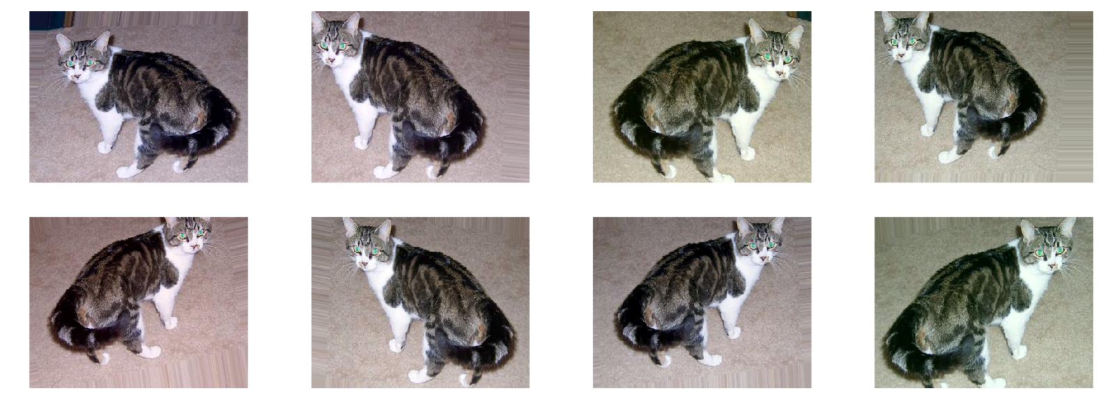
Data augmentation includes things like randomly rotating the image, zooming in, adding a color filter etc. Data augmentation only happens to the training set and not on the validation/test set. It can be useful to check if you are using too much data augmentation. For example, if you zoom in so much that features of a cat are not visible anymore, than the model is not going to get better from training on these images. Let’s explore some data augmentation!

For followers of the Fast AI course: be aware that the notebook uses ‘width_zoom_range’ as one of the data augmentation arguments. However, this option is not available anymore in Keras.

Let’s now have a look at the image after performing data augmentation. All of the ‘cats’ are still clearly recognizable as cats to me.

The third step is to use an architecture that generalizes well. However, much more important is the fourth step: adding regularization. The three most popular options are: dropout, L1 regularization and L2 regularization. In deep learning you will mostly see dropout, which I discussed earlier. Dropout deletes a random sample of the activations (makes them zero) in training. In the Vgg model this is only applied in the fully connected layers at the end of the model. However, it can also be applied to the convolutional layers. Be aware that dropout causes information to get lost. If you lose something in the first layer, it gets lost for the whole network. Therefore, a good practice is to start with a low dropout in the first layer and then gradually increase it. The fifth and final option is to reduce the network complexity. In reality, various forms of regularization should be enough to deal with overfitting in most cases.

Batch Normalization

Finally, let’s discuss batch normalization. This is something you should always do! Batch normalization is a relatively new concept and therefore was not yet implemented in the Vgg model.

Standardizing the inputs of your model is something that you have definitely heard about if you are into machine learning. Batch normalization takes this a step further. Batch normalization adds a ‘normalization layer’ after each convolutional layer. This allows the model to converge much faster in training and therefore also allows you to use higher learning rates.

Simply standardizing the weights in each activation layer will not work. Stochastic Gradient Descent is very stubborn. If wants to make one of the weights very high it will simply do it the next time. With batch normalization the model learns that it can adjust all the weights instead of one each time.

MNIST Digit Recognition

The MNIST handwritten digits dataset is one of the most famous datasets in machine learning. The dataset also is a great way to experiment with everything we now know about CNNs. Kaggle also hosts the MNIST dataset. This code I quickly wrote is all that is necessary to score 96.8% accuracy on this dataset.

import pandas as pd
from sklearn.ensemble import RandomForestClassifier

train = pd.read_csv('train_digits.csv')
test = pd.read_csv('test_digits.csv')

X = train.drop('label', axis=1)
y = train['label']

rfc = RandomForestClassifier(n_estimators=300)
pred = rfc.fit(X, y).predict(test)

However, fitting a deep CNN can get this result up to 99.7%. This week I will try to apply a CNN to this dataset and hopefully next week I can report the accuracy I reached and discuss the issues I ran into.

If you liked this posts be sure to recommend it so others can see it. You can also follow this profile to keep up with my process in the Fast AI course. See you there!