自编码器

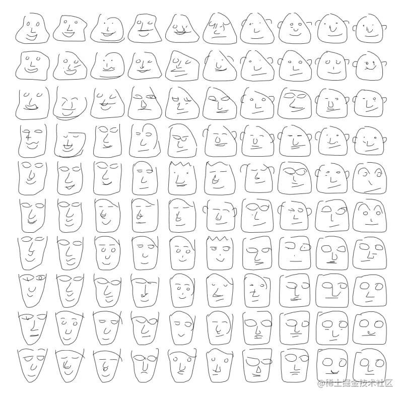
自编码器，可以进行无监督的特征学习，可以将高维数据压缩并重构。

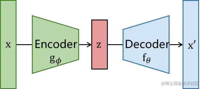
Autoencoder可以使用无标签数据训练，将数据压缩到潜变量空间上。但是仅有一个编码器和输入数据我们无法训练获得$\mathbf z$，因此我们加一个解码器重构数据为$\hat{\mathbf x}$，保证${\mathbf x}$和$\hat{\mathbf x}$越接近越好，就可以证明$\mathbf z$中保留了${\mathbf x}$的特征。这样Autoencoder就实现了编码器解码器的联合训练。

输入样本${\mathbf x}$通过编码器获得低维特征$\mathbf z$，最后通过解码器重构输入数据获得$\hat{\mathbf x}$，loss直接最小化$||\mathbf x-\hat{\mathbf x}||^2$即可实现无监督训练。

.

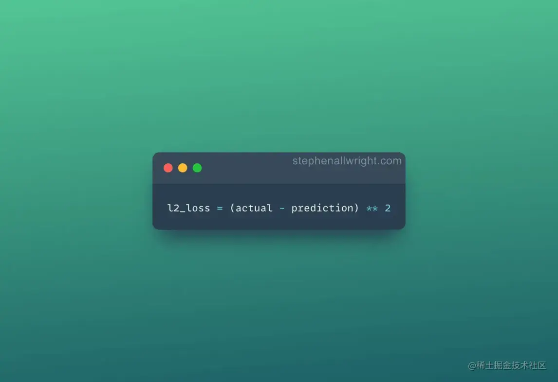
数学公式好好写一下AE的目标函数：

这里就是用了个MSE loss。

一个训练好的AE：

• 编码器：特征提取 将数据$\mathbf x$输编码器，提取特征，得到bottleneck层的潜变量表示$\mathbf z$
• 解码器：生成器 使用潜变量$\mathbf z$，重建数据。

学习完成之后，解码器就可以做图片生成器。在低维空间上非编码处进行解码可以生成新的不同于输入的样本。

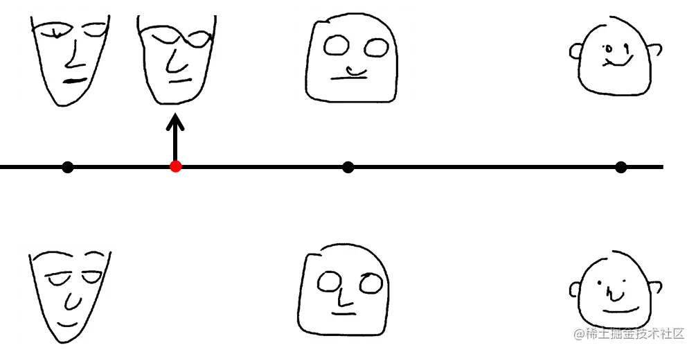
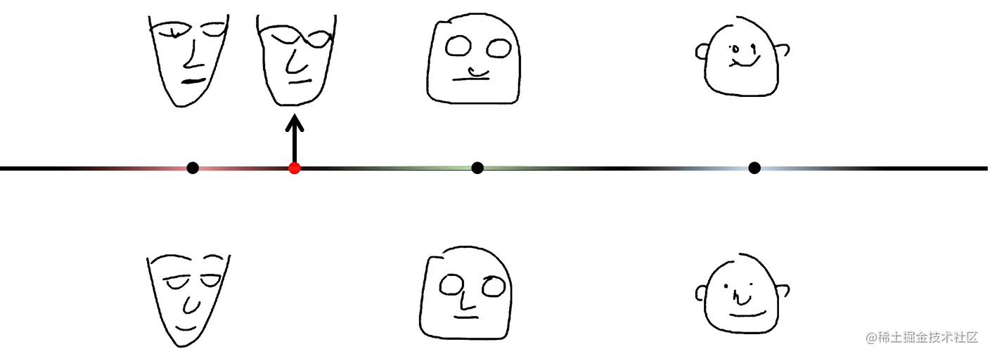
比如上图，中间这条线假设是我们学习到的码空间，下边的三个人脸是输入数据，上边的三个人脸是对应的重建输出。现在我们采样橙色那个点，你可能会想，它应该可以生成介于尖脸和方脸之间的一种脸型。但是实际上AE是做不到这一点的。

问题在于因为神经网络只是稀疏地记录下来你的输入样本和生成图像的一一对应关系，所以，如果介于某两个特征之间的某个点，编码器并没有学习到码空间里。因此无法实现码空间随机采样即可生成对应的图片，随机采样的点在解码时一定不会生成我们所希望特征的图像。

码空间的泛化能力基本为零，所以AE模型训练出来的解码器存在缺陷。

所以你采样红色的点的时候，解码器会说：啊？编码器没告诉过我啊。 所以是AE生成不出你期望的东西的。那怎么办呢？我们可以使用VAE。

VAE

为什么VAE可以做到？

原来的AE是将输入映射到固定向量，现在VAE的要求是将其映射到分布中，也就是给原来的固定点引入噪音，你要在这个噪声的范围的都能重建回这个图像。将原来的一个点变成了一个范围。

那当我们取某一个点的时候，它同时被不同的区间覆盖到，所以当它要生成一个东西的时候会产生介于二者之间的结果，使用VAE我们就可以获得在尖脸和方脸之间的结果了。

VAE的结构

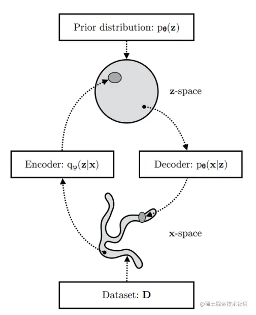
我们看一下作者画的图：

我们有一个数据集$\mathrm D$，它的分布是未知的。也就是图中的$\mathbf x$space。通过VAE的编码器之后将其压缩到潜变量空间$\mathbf z$space上了。VAE的解码器要使用能从$\mathbf z$space上采样点，生成$\mathbf x'$，要让$\mathbf x'$尽力和$\mathbf x$相似。如果成功的话，那$\mathbf x'$的空间应该和和$\mathbf x$差不多。

解码器

解码器的作用是从$\mathbf z$space上采样点，然后重建$\mathbf x$space：

1. 首先，从先验分布 $p_\theta(\mathbf{z})$ 中采样一个 $\mathbf{z}^{i}$。
2. 然后从条件分布 $p_\theta \left(\mathbf{x} \mid \mathbf{z}=\mathbf{z}^{i}\right)$ 中生成一个值 $\mathbf{x}^{i}$。

最优参数 $\theta^*$ 是最大化生成真实数据样本概率的参数，也就是计算$p_\theta(\mathbf x)$的极大似然：

$\theta^* =\arg \max \theta \prod_{i=1}^n p_\theta\left(\mathbf{x}^{i}\right)$

通常我们使用对数概率将右侧的乘积转换为求和：

$\theta^*=\arg \max \theta \sum_{i=1}^n \log p_\theta\left(\mathbf{x}^{i}\right)$

编码器

我们看一下$p_\theta\left(\mathbf{x}^{i}\right)$是怎么出来的： $p_\theta\left(\mathbf{x}^{i}\right)=\int p_\theta\left(\mathbf{x}^{i} |\mathbf{z}\right) p(\mathbf{z}) d \mathbf{z}$ 我们可以发现这样计算 $p_\theta\left(\mathbf{x}^{i}\right)$ 并不容易，因为不可能检查所有的 $\mathbf{z}$ 值。

为了缩小值空间， 我们现在这样考虑：无法计算所有的$\mathbf z$，那我们只计算给定对应的$\mathbf x$的时候能出现什么样的$\mathbf z$，然后再看$\mathbf z$能否重建回$\mathbf x$不就行了。

那如何获得后验$p_\theta(\mathbf z | \mathbf x)$，这就引入网络的编码器了。 我们引入一个新的近似函数 $q_\phi(\mathbf{z} |\mathbf{x})$，用于估计给定输入 $\mathbf{x}$ 时可能的编码，也就是用$q_\phi(\mathbf{z}|\mathbf{x})$去近似真实后验$p_\theta(\mathbf z | \mathbf x)$。

现在，结构看起来很像一个自编码器：

条件概率 $p_\theta(\mathbf{x} \mid \mathbf{z})$ 定义了一个生成模型，类似于上面介绍的AE解码器 $f_\theta(\mathbf{x} \mid \mathbf{z})$，$p_\theta(\mathbf{x} \mid \mathbf{z})$ 也被称为概率解码器。

近似函数 $q_\phi(\mathbf{z} \mid \mathbf{x})$ 是概率编码器，扮演了AE中 $g_\phi(\mathbf{z} \mid \mathbf{x})$ 相似的角色。

到这里就回到了本节开头作者画的那张图了。

目标函数

估计的后验 $q_\phi(\mathbf{z} \mid \mathbf{x})$ 应该非常接近真实的后验 $p_\theta(\mathbf{z} \mid \mathbf{x})$。我们可以使用 KL散度来量化这两个分布之间的距离。

现在我们来将这个KL散度展开计算：

$\begin{aligned} & D_{\mathrm{KL}}\left(q_\phi(\mathbf{z} \mid \mathbf{x}) \| p_\theta(\mathbf{z} \mid \mathbf{x})\right) \\ & =\int q_\phi(\mathbf{z} \mid \mathbf{x}) \log \frac{q_\phi(\mathbf{z} \mid \mathbf{x})}{p_\theta(\mathbf{z} \mid \mathbf{x})} d \mathbf{z} \\ & =\int q_\phi(\mathbf{z} \mid \mathbf{x}) \log \frac{q_\phi(\mathbf{z} \mid \mathbf{x}) p_\theta(\mathbf{x})}{p_\theta(\mathbf{z}, \mathbf{x})} d \mathbf{z} &因为 p(z, x)=p(x \mid z) p(z) \\ & =\int q_\phi(\mathbf{z} \mid \mathbf{x})\left(\log p_\theta(\mathbf{x})+\log \frac{q_\phi(\mathbf{z} \mid \mathbf{x})}{p_\theta(\mathbf{z}, \mathbf{x})}\right) d \mathbf{z} \\ & =\log p_\theta(\mathbf{x})+\int q_\phi(\mathbf{z} \mid \mathbf{x}) \log \frac{q_\phi(\mathbf{z} \mid \mathbf{x})}{p_\theta(\mathbf{z}, \mathbf{x})} d \mathbf{z} & 因为\int q(z \mid x) d z=1 \\ & =\log p_\theta(\mathbf{x})+\int q_\phi(\mathbf{z} \mid \mathbf{x}) \log \frac{q_\phi(\mathbf{z} \mid \mathbf{x})}{p_\theta(\mathbf{x} \mid \mathbf{z}) p_\theta(\mathbf{z})} d \mathbf{z} & 因为p(z, x)=p(x \mid z) p(z) \\ & =\log p_\theta(\mathbf{x})+\mathbb{E}_{\mathbf{z} \sim q_\phi(\mathbf{z} \mid \mathbf{x})}\left[\log \frac{q_\phi(\mathbf{z} \mid \mathbf{x})}{p_\theta(\mathbf{z})}-\log p_\theta(\mathbf{x} \mid \mathbf{z})\right] \\ & =\log p_\theta(\mathbf{x})+D_{\mathrm{KL}}\left(q_\phi(\mathbf{z} \mid \mathbf{x}) \| p_\theta(\mathbf{z})\right)-\mathbb{E}_{\mathbf{z} \sim q_\phi(\mathbf{z} \mid \mathbf{x})} \log p_\theta(\mathbf{x} \mid \mathbf{z}) \end{aligned}$

现在得到：

$D_{\mathrm{KL}}\left(q_\phi(\mathbf{z} \mid \mathbf{x}) \| p_\theta(\mathbf{z} \mid \mathbf{x})\right)=\log p_\theta(\mathbf{x})+D_{\mathrm{KL}}\left(q_\phi(\mathbf{z} \mid \mathbf{x}) \| p_\theta(\mathbf{z})\right)-\mathbb{E}_{\mathbf{z} \sim q_\phi(\mathbf{z} \mid \mathbf{x})} \log p_\theta(\mathbf{x} \mid \mathbf{z})$

移项：

$\log p_\theta(\mathbf{x})-D_{\mathrm{KL}}\left(q_\phi(\mathbf{z} \mid \mathbf{x}) \| p_\theta(\mathbf{z} \mid \mathbf{x})\right)=\mathbb{E}_{\mathbf{z} \sim q_\phi(\mathbf{z} \mid \mathbf{x})} \log p_\theta(\mathbf{x} \mid \mathbf{z})-D_{\mathrm{KL}}\left(q_\phi(\mathbf{z} \mid \mathbf{x}) \| p_\theta(\mathbf{z})\right)$

• 先看方程右边：

  $\mathbb{E}_{\mathbf{z} \sim q_\phi(\mathbf{z} \mid \mathbf{x})} \log p_\theta(\mathbf{x} \mid \mathbf{z})-D_{\mathrm{KL}}\left(q_\phi(\mathbf{z} \mid \mathbf{x}) \| p_\theta(\mathbf{z})\right)$

  • 第一项可以认为是重建项：我们先从变分分布中采样$\mathbf{z} \sim q_\phi(\mathbf{z} \mid \mathbf{x})$，然后用解码器将其解码。

  • 第二项可以认为是先验匹配项：我们学到的分布和先验的相似程度。

  当我们尽力最大化这一项的时候，就是让第一项尽量大，让第二项尽量小，这就意味着：

  • 第一项是让解码器尽量去从变分分布中重建数据。

  • 第二项是让编码器去学习一个实际分布，让变分分布和先验更相似，而不是崩溃侧灰姑娘delta函数。

• 再看方程的左边：

  $\log p_\theta(\mathbf{x})-D_{\mathrm{KL}}\left(q_\phi(\mathbf{z} \mid \mathbf{x}) \| p_\theta(\mathbf{z} \mid \mathbf{x})\right)$

  • 第一项是我们在学习真实分布时想要最大化生成真实数据的（对数）似然。

  • 第二项是真实后验和近似后验分布之间的差异（这个KL散度项在这是起到正则化的作用）。

  • 注意 $p_\theta(\mathbf{x})$ 关于 $q_\phi$ 是固定的。

  最大化这一项就是：

  • 最大化生成真实数据的（对数）似然。

  • 让真实后验和近似后验之间的差异尽量小。

上面的式子取反之后定义了我们的损失函数：

$\begin{aligned} L_{\mathrm{VAE}}(\theta, \phi) & =-\log p_\theta(\mathbf{x})+D_{\mathrm{KL}}\left(q_\phi(\mathbf{z} \mid \mathbf{x}) \| p_\theta(\mathbf{z} \mid \mathbf{x})\right) \\ & =-\mathbb{E}_{\mathbf{z} \sim q_\phi(\mathbf{z} \mid \mathbf{x})} \log p_\theta(\mathbf{x} \mid \mathbf{z})+D_{\mathrm{KL}}\left(q_\phi(\mathbf{z} \mid \mathbf{x}) \| p_\theta(\mathbf{z})\right) \end{aligned}$

$\theta^*, \phi^* =\arg \min _{\theta, \phi} L_{\mathrm{VAE}}$

在变分贝叶斯方法中，这个损失函数被称为变分下界，或证据下界。

因为KL 散度总是非负的，因此$-L_{\mathrm{VAE}}$ 是 $\log p_\theta(\mathbf{x})$ 的下界。

$\log p_\theta(\mathbf{x}) \geq -L_{\mathrm{VAE}}=\log p_\theta(\mathbf{x})-D_{\mathrm{KL}}\left(q_\phi(\mathbf{z} \mid \mathbf{x}) \| p_\theta(\mathbf{z} \mid \mathbf{x})\right)$

因此，通过最小化损失，我们也就是在最大化生成真实数据样本概率的下界。

参数重整化

因为$\mathbf{z} \sim q_\phi(\mathbf{z} \mid \mathbf{x})$这里采样$\mathbf z$具有随机性，无法使用网络的梯度传播，因此作者使用参数重整化技巧转嫁随机性。之后网络结构如下：

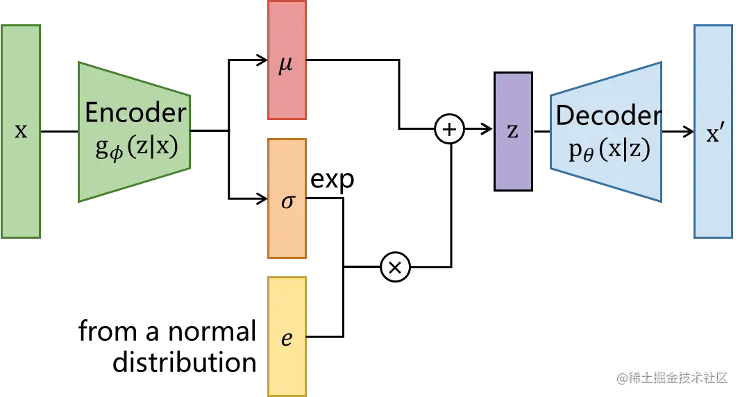
之后就可以快乐地生成人脸了！