本文已参与「新人创作礼」活动,一起开启掘金创作之路。
定积分的几何应用
一、平面图形的面积
1. 直角坐标
-
由曲线y=f(x)(f(x)≥0)及直线x=a,x=b(a<b)与x轴所围成的曲面梯形的面积A是定积分A=∫abf(x)dx
-
由曲线y=f(x)(f(x)≤0)及直线x=a,x=b(a<b)与x轴所围成的曲面梯形的面积A是定积分A=−∫abf(x)dx
-
由曲线y=f(x),y=g(x)(f(x)≤g(x))及直线x=a,x=b(a<b)与x轴所围成的曲面梯形的面积A是定积分A=∫ab[g(x)−f(x)]dx
-
由曲线y=f(x),y=g(x)(f(x)≥g(x))及直线x=a,x=b(a<b)与x轴所围成的曲面梯形的面积A是定积分A=∫ab[f(x)−g(x)]dx
例1:计算抛物线:y2=x,y=x2所围成图形的面积
一定要画图(本节笔记都有图,其他笔记如有必要会进行展示)
导包以及直角坐标系的通用设置(不同会特别说明)
import numpy as np

import matplotlib.pyplot as plt

plt.rcParams['figure.figsize']=(8,6)

ax=plt.gca()

ax.spines['right'].set_color('none')

ax.spines['top'].set_color('none')

ax.spines['bottom'].set_position(('data', 0))

ax.spines['left'].set_position(('data',0))

ax.set_aspect(1)
X=np.arange(-5,5,0.002)

f1=lambda x:x**2

f2=lambda x:x**0.5

f3=lambda x:-x**0.5

s1=pd.Series(f1(X),index=X)

s2=pd.Series(f2(X),index=X)

s3=pd.Series(f3(X),index=X)

s1.plot()

s2.plot(color='orange')

s3.plot(color='orange')

plt.ylim(-2,2)

plt.xlim(-1,2)
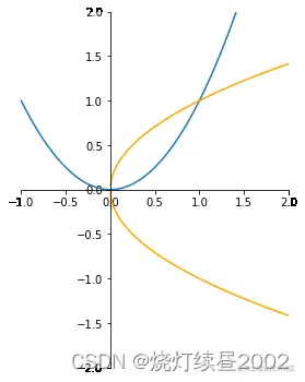
dA=(x−x2)dx
联立{y2=xy=x2解得{x=0y=0或{x=1y=1
A=∫01(x−x2)dx=(32x23−31x3)∣∣01=31
例2:计算抛物线y2=2x与直线y=x−4所围成的图形的面积
X=np.arange(-5,10,0.002)

f1=lambda x:2**0.5*x**0.5

f2=lambda x:-2**0.5*x**0.5

f3=lambda x:x-4

s1=pd.Series(f1(X),index=X)

s2=pd.Series(f2(X),index=X)

s3=pd.Series(f3(X),index=X)

s1.plot(color='orange')

s2.plot(color='orange')

s3.plot()

plt.ylim(-5,5)
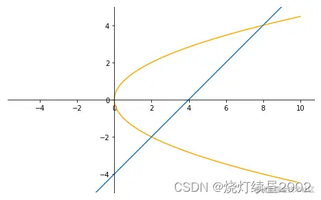
联立{y2=2xy=x−4解得{x=8y=4或{x=2y=−2
对x轴积分
dA1=(2x+2x)dx(x∈(0,2)),dA2=(2x−x+4)dx(x∈(2,8))
A=∫0222xdx+∫28(2x−x+4)dx
对y轴积分同理
dA=(4+y−2y2)dy
A=∫−24(4+y−2y2)dy=(4y+21y2−61y3)∣−24=18
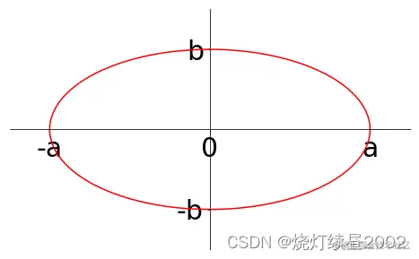
例3:求椭圆a2x2+b2y2=1所围成的图形的面积
此处画图以a=2,b=1为例,设置轴标签变换的图像。以后凡是涉及参数大都是这种思路
theta=np.arange(0,2*np.pi,0.01)

a=2

b=1

f=lambda theta:a*np.cos(theta),lambda theta:b*np.sin(theta)

plt.plot(f[0](theta),f[1](theta),color='r')

plt.ylim(-1.5,1.5)

plt.xlim(-2.5,2.5)

plt.xticks([-2,2])

plt.yticks([-1,1])

ax.set_xticklabels(['-a','a'],fontsize=30)

ax.set_yticklabels(['-b','b'],fontsize=30)
法1:
由于图像关于x,y轴均对称,因此计算第一象限面积再乘4
参数方程
令{x=acosty=bsint
(0≤t≤2π)
dA=4dA1=4ydx=4yd(acost=4bsintd(acost)=−4absin2tdt
A=−4ab∫2π0sin2tde=πab
法2:
dA=4dA1=4y(x)dx=4aba2−x2dx
A=4ab∫0aa2−x2dxdx=acostdt=令x=asint4ab∫02πa2cos2tdt=4ab∫02πcos2tdt=πab
2. 极坐标
设由曲线ρ=ρ(θ)及射线θ=α,θ=β围成的一个图形,这个曲边扇形的面积A是定积分A=∫αβ21[ρ(θ)]2dθ
例1:计算阿基米德螺线ρ=αθ(α>0)上相应于θ从0变到2π的一段弧与极轴所围成的图形的面积
theta=np.arange(0,2*np.pi,0.02)
a=1
f=lambda theta:a*theta
ax=plt.gca(projection='polar')
plt.plot(theta,f(theta))
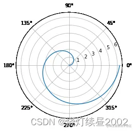
dA=21ρ2dθ=21a2θ2dθ
A=∫02π21a2θ2dθ=2a2(31θ3)∣02π=34π3a2
例5:计算心形线ρ=a(1+cosθ)(a>0)所围成图形的面积
theta=np.arange(0,2*np.pi,0.02)

a=5

f=lambda theta:a*(1+np.cos(theta))

ax=plt.gca(projection='polar')

plt.plot(theta,f(theta))
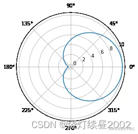
dA=2(21ρ2dθ)=2(21a2(1+cosθ)2)dθ
可选择(0,π)再乘2,也可直接选择(0,2π),二者同理
A=∫0πa2(1+cosθ)2dθ=a2∫0π(1+2cosθ+cos2θ)dθ(结合图像发现cosθ在(0,2π)上x轴上下面积相等)=a2∫0πdθ+2a2∫02πcos2θdθ(结合图像,换到(0,2π)区间上)=23πa2
见到区间长度是2π的整数倍,积分中含有sin,cos,结合图像可以缩小区间或者发现积分为0
二、旋转体的体积
设连续曲线y=f(x)、直线x=a,x=b及x轴所围成的曲边梯形绕x轴旋转一周所围成的旋转体的体积,体积微元是dV=π[f(x)]2dx,体积是V=∫abπ[f(x)]2dx
例6:连接坐标原点O及点P(h,r)的直线、直线x=h及x轴围成一个直角三角形,将它绕x轴旋转一周构成一个底面半径为r、高为h的圆锥体,计算该圆锥体的体积
dV=πy2(x)dx=π(hrx)2dx
V=π(hr)2∫0hx2dx=3πr2h
例7:计算由摆线x=a(t−sint),y=a(1−cost)相应于0≤t≤2π的一拱与直线y=0所围成的图形分别绕x轴与y轴旋转一周而成的旋转体的体积
theta=np.arange(-1*np.pi,3*np.pi,0.02)

a=1

f=lambda theta:a*(theta-np.sin(theta)),lambda theta:a*(1-np.cos(theta))

plt.plot(f[0](theta),f[1](theta))

plt.xticks([0,2*np.pi])

plt.yticks([2])

ax.set_xticklabels([0,'2πa'])

ax.set_yticklabels(['2a'])
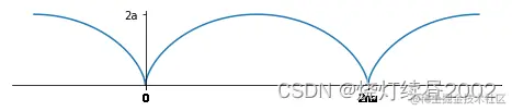
参数方程根据x或y的极值或零点,确定t的值,从而确定y或x的值,最终确定直角坐标系上的坐标
dVx=πy2(x)dx=πy2(t)x′(t)dt=πa2(1−cost)2⋅a(1−cost)dt
Vx=∫02ππa3(1−cost)3dt=πa3∫02π(1−3cost+3cos2t−cos3t)dt=5π2a3
dVy1=πx12(y)dy=π[a(t−sint)]2⋅asintdt
dVy2=πx22(y)dy=π[a(t−sint)]2⋅asintdt
Vy=∫02aπx12(y)dy−∫02aπx12(y)dy虽然都是∫02a,但第一个式子是x∈(πa,2πa)曲线与y轴构成的面,第二个式子是x∈(0,πa)曲线与y轴构成的面,二者相减得到的结果对于第一个式子的下限0,根据y=a(1−cost)得t=2π。其余上下限转化同理=π∫2ππ[a(t−sint)]2⋅asintdt−π∫0π[a(t−sint)]2⋅asintdt=−π∫02πa3(t−sint)2sintdt=6π3a3
三、平面曲线的弧长
1. 直角坐标
当曲线弧由直角坐标方程y=f(x)(a≤x≤b)确定,其中f(x)在其闭区间[a,b]上具有一阶连续导数,则曲线弧长为s=∫ab1+y′2(x)dx
推导:
(ds)2=(dx)2+(dy)2
ds=(dx)2+(dy)2=1+(dxdy)2dx=1+y′2(x)dx
2. 参数方程
当曲线弧由参数方程{x=x(t)y=y(t)(α≤t≤β)确定,其中x=x(t)与y=y(t)在闭区间t∈[α,β]具有连续导数,所以曲线弧长为s=∫αβx′2(t)+y′2(t)dt
推导:
(ds)2=(dx)2+(dy)2
ds=(dx)2+(dy)2=(dtdx)2+(dtdy)2dt=x′2(t)+y′2(t)dt
3. 极坐标
当曲线弧由极坐标方程ρ=ρ(θ)(α≤θ≤β)确定,其中ρ(θ)在闭区间[α,β]上具有连续导数,则由直角坐标与极坐标的关系得知{x=x(θ)=ρ(θ)cosθy=y(θ)=ρ(θ)sinθ(α≤θ≤β),极坐标其实就是以极角θ为参数的曲线弧的参数方程,所以曲线弧长为s=∫αβρ2(θ)+ρ′2(θ)dθ
推导:
ds=x′2(θ)+y′2(θ)dθ=(ρ′cosθ−ρsinθ)2+(ρ′sinθ+ρcosθ)2dθ=ρ2(sin2θ+cos2θ)+ρ′2(sin2θ+cos2θ)dθ=ρ2(θ)+ρ′2(θ)dθ
例8:求阿基米德螺线ρ=aθ(a>θ)相应于0≤θ≤2π的一段弧长
ds=ρ2(θ)+ρ′2(θ)dθ=a1+θ2dθ
s=a∫02π1+θdθ=a[2θ1+θ2+21ln(θ+1+θ2)]∣∣02π=π1+4π2+21ln(2π+1+4π2)
这个积分不容易计算,可以先换成不定积分进行计算,不定积分积完后代入上下限。注意,这种方法的前提是,被积函数在积分区间上连续,如不连续,可以分区间再用该种方法
∫x2+a2dxdx=asec2udu=x=atanu∫asecu⋅asec2udu(1)=a2∫secudtanu=a2secutanu+a2∫tan2usecudu=a2secutanu+a2∫(sec3u−secu)du=a2secutanu−a2ln∣secu+tanu∣+a2∫sec3udu(2)
(1)(2)凑成循环积分,因此
∫x2+a2dxdx=asec2udu=x=atanu2a2tanusecu+2a2ln∣secu+tanu∣+C
代回x
∫x2+a2dx=2xx2+a2+21ln(x+x2+a2)+C
定积分在物理学上的应用
一、变力沿直线做功
公式:W=F⋅s
例1:一圆柱形的储水桶高为5m,底圆半径为3m,桶内盛满了水,试问要把桶内的水全部吸出需做多少功
建系如图
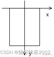
dW=dF⋅s=dm⋅gy=ρdV⋅gy=ρgyπ32dy=9πρgydy
W=9πρg∫05ydy=2225πρg(J)
二、水压力
公式:P=p⋅A=ρgh⋅A
其中水的密度为ρ,重力加速度为g,h为离水面的深度,A为放置在水深为h的物体的面积
例2:一个横放着的圆柱形水桶,桶内盛有半桶水,设桶的底半径为R,水的密度为ρ,计算桶的一个端面(圆面)上所受的压力
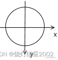
dP=pdA=ρgydA=ρgy⋅2x(y)dy=2ρgyR2−y2dy
P=2ρg∫0RyR2−y2dy=−ρg[32(R2−y2)23]∣∣0R=32ρgR3


