如何用Sklearn GridSearchCV和RandomizedSearchCV进行超参数调控

简介

在这篇文章中，我们将向你解释Sklearn的一个非常有用的模块 - GridSearchCV。 我们将首先了解什么是GridSearchCV，它有什么好处。然后，我们将带你看一些GridSearchCV的各种例子，如Logistic Regression、KNN、Random Forest和SVM的算法。最后，我们还将讨论RandomizedSearchCV以及一个例子。

什么是GridSearchCV？

GridSearchCV是Sklearn model_selection包的一个模块，用于超参数调整。给定一组不同的超参数，GridSearchCV 循环浏览所有可能的超参数值和组合，并在训练数据集上拟合模型。在这个过程中，它能够确定产生最佳精度的超参数的最佳值和组合（从给定的参数集中）。

为什么我们需要GridSearchCV？

通常情况下，我们所做的是根据直觉或经验来选择超参数，或者甚至只是胡乱猜测。

通常情况下，一开始，我们只是凭直觉或计算猜测来提供ML算法的超参数值。如果准确率不高，我们就会手动尝试其他超参数的值和组合。但这个手动过程可能是相当耗时的，你甚至可能无法涵盖所有的组合，或者中途放弃。

这时，Sklearn GridsearchCV就可以很好地将这个手工工作自动化。你可以提供不同的超参数列表，它将为你做繁重的工作并返回最佳的超参数组合和模型作为输出。

GridSearchCV是如何工作的？

我们把一组超参数的值作为字典传给GridSearchCV函数。例如，在SVM（支持向量机）中，超参数的提供方式是------。

{ 'C':[0.1, 1, 10, 100], 'gamma':[1, 0.1, 0.01, 0.001, 0.0001], 'kernel':['rbf', 'linear', ' poly']}。

这里C、gamma和kernel是SVM模型的可能超参数。

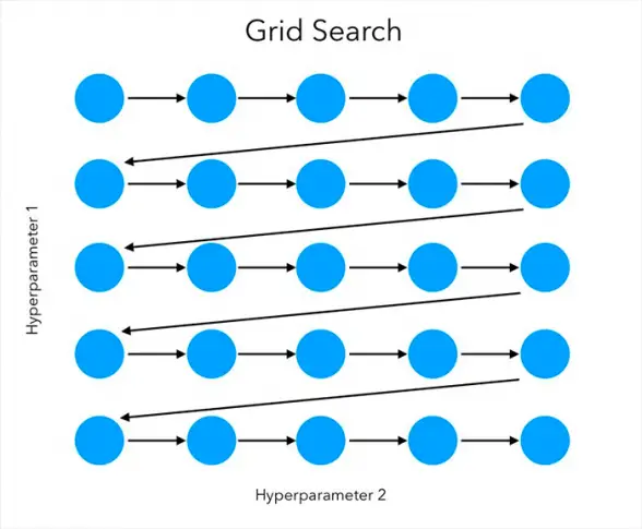
超参数被设置在一个离散的网格中，然后它使用网格中的每个值的组合，使用交叉验证来评估性能。在交叉验证中使平均值最大化的网格点，就是超参数值的最佳组合。

(来源)

Sklearn GridSearchCV函数的常用参数

• 估计器：这里我们传入我们的模型实例。
• params_grid：它是一个字典对象，用来保存我们想要实验的超参数。
• scoring: 我们想要实现的评估指标，例如Accuracy,Jaccard,F1macro,F1micro。
• cv：我们对每个超参数进行交叉验证的总次数。
• verbose。详细打印出你对GridSearchCV的数据拟合，大多数情况下我们将其设置为1。
• n_jobs: 你希望在这个任务中并行运行的进程数，如果它是-1，它将使用所有可用的处理器。

Sklearn GridSearchCV的例子

我们将使用一个银行客户流失的数据集来向你展示Sklearn GridSearchCV在以下算法中的例子

• Logistic回归
• KNN
• 随机森林
• SVM

关于我们的数据集

该数据集包含银行客户流失的详细信息。客户流失是指客户停止与公司的关系。我们的目标是创建一个机器学习模型来预测客户是否会离开银行服务。该数据集由1000行和14列组成。

导入必要的库

我们首先加载建立模型所需的库。

在[3]中：

#import all necessary libraries
import numpy as np 
import pandas as pd 
import seaborn as sns
import matplotlib.pyplot as plt
from sklearn.metrics import accuracy_score, plot_confusion_matrix
from sklearn.model_selection import GridSearchCV

读取CSV文件

现在我们将数据集的CSV文件加载到Pandas Dataframe中。

在[4]中：

df=pd.read_csv(r"Churn_Modelling.csv")

现在让我们看看关于我们的数据的一些汇总统计，这将包括关于列数据类型的信息，它们的计数，此外，我们还将显示汇总统计，如平均值，最小值和最大值，平均值和标准差。

In[6]:

df.info()

输出[6]：

<class 'pandas.core.frame.DataFrame'>
RangeIndex: 10000 entries, 0 to 9999
Data columns (total 14 columns):
 #   Column           Non-Null Count  Dtype  
---  ------           --------------  -----  
 0   RowNumber        10000 non-null  int64  
 1   CustomerId       10000 non-null  int64  
 2   Surname          10000 non-null  object 
 3   CreditScore      10000 non-null  int64  
 4   Geography        10000 non-null  object 
 5   Gender           10000 non-null  object 
 6   Age              10000 non-null  int64  
 7   Tenure           10000 non-null  int64  
 8   Balance          10000 non-null  float64
 9   NumOfProducts    10000 non-null  int64  
 10  HasCrCard        10000 non-null  int64  
 11  IsActiveMember   10000 non-null  int64  
 12  EstimatedSalary  10000 non-null  float64
 13  Exited           10000 non-null  int64  
dtypes: float64(2), int64(9), object(3)
memory usage: 1.1+ MB

我们需要去掉一些不相干的特征，这些特征在我们的预测中不会用到，因此我们使用删除法来删除某些不必要的列。

在[9]中：

df.drop(['RowNumber', 'CustomerId', 'Surname', 'Geography'], axis=1, inplace=True)

df.Gender = [1 if each == 'Male' else 0 for each in df.Gender]

在[10]中：

df.head()

Out[10]:

	信用分数	性别	年龄	任期	帐户余额	产品数量	有卡	是活跃会员	薪资估计	已退出
0	619	0	42	2	0.00	1	1	1	101348.88	1
1	608	0	41	1	83807.86	1	0	1	112542.58	0
2	502	0	42	8	159660.80	3	1	0	113931.57	1
3	699	0	39	1	0.00	2	0	0	93826.63	0
4	850	0	43	2	125510.82	1	1	1	79084.10

将数据集分割成训练集和测试集

接下来，我们将独立预测变量和目标变量分成x和y，然后在train_test_split()函数的帮助下将x和y分成训练集和测试集。

在[14]中：

from sklearn.model_selection import train_test_split 

x=df.drop('Exited', axis=1)

y = df['Exited']

x_train, x_test, y_train, y_test = train_test_split(x, y, test_size=0.20, random_state=7)

使用GridSearchCV的Logistic回归

现在我们将向你展示一个使用 GridSearchCV 进行逻辑回归的例子。

在[18]中：

# Grid search cross validation

from sklearn.linear_model import LogisticRegression
grid={"C":np.logspace(-3,3,20), "penalty":["l2"]} 
logreg=LogisticRegression()
grid_logreg=GridSearchCV(logreg,grid,cv=10)
grid_logreg.fit(x_train,y_train)

print("tuned hpyerparameters :(best parameters) ",grid_logreg.best_params_)
print("accuracy :",grid_logreg.best_score_*100)

Out[18]:

tuned hpyerparameters :(best parameters)  {'C': 0.00206913808111479, 'penalty': 'l2'}
accuracy : 79.06249999999999

在[19]中：

# make predictions on test data 
grid_predictions = grid_logreg.predict(x_test) 

test_accuracy=accuracy_score(y_test,grid_predictions)*100
print("Accuracy for our testing dataset with tuning is : {:.2f}%".format(test_accuracy) )

Out[19]:

Accuracy for our testing dataset with tuning is : 78.85%

• 还可以阅读 - Python Sklearn Logistic Regression 教程与实例

使用GridSearchCV的KNN

接下来，我们向你展示一个使用GridSearchCV与KNN算法的例子。

In[23]:

k_range = list(range(1, 31))
param_grid = dict(n_neighbors=k_range)
grid_knn = GridSearchCV(knn, param_grid, cv=5, scoring='accuracy', return_train_score=False)
grid_knn.fit(x_train,y_train)
print("tuned hyperparameters :(best parameters) ",grid_knn.best_params_)
print("accuracy :",grid_knn.best_score_*100)

Out[23]:

tuned hyperparameters :(best parameters)  {'n_neighbors': 30}
accuracy : 79.66250000000001

In [24]:

# make predictions on test data 
grid_predictions = grid_knn.predict(x_test) 
test_accuracy=accuracy_score(y_test,grid_predictions)*100
print("Accuracy for our testing dataset with tuning is : {:.2f}%".format(test_accuracy) )

Out[24]:

Accuracy for our testing dataset with tuning is : 79.45%

• 还可以阅读 - 在Sklearn中使用GridSearchCV的KNN分类器与实例

使用 GridSearchCV 的随机森林

现在我们将向你展示一个使用GridSearchCV与随机森林的例子。

In[29]:

param_grid = {
    'n_estimators': [200, 700],
    'max_features': ['auto', 'sqrt', 'log2']
}
CV_rfc = GridSearchCV(estimator=rf,param_grid=param_grid, cv= 5,scoring='accuracy')
CV_rfc.fit(x_train, y_train)
print("tuned hyperparameters :(best parameters) ",CV_rfc.best_params_)
print("accuracy :",CV_rfc.best_score_*100)

Out[29]:

tuned hyperparameters :(best parameters)  {'max_features': 'log2', 'n_estimators': 700}
accuracy : 85.3

In [30]:

# make predictions on test data 
grid_predictions = CV_rfc.predict(x_test) 
test_accuracy=accuracy_score(y_test,grid_predictions)*100
print("Accuracy for our testing dataset with tuning is : {:.2f}%".format(test_accuracy) )

Out[30]:

Accuracy for our testing dataset with tuning is : 84.90%

• 还可以阅读 - Python Sklearn中的随机森林分类器与实例

使用GridSearchCV的SVM

最后，我们有一个使用 GridSearchCV 与 SVM 的例子。

In[34]:

# defining parameter range
param_grid = {'C': [0.1, 1, 10, 100, 1000], 
              'gamma': [1, 0.1, 0.01, 0.001, 0.0001],
              'kernel': ['rbf']} 
  
grid = GridSearchCV(svm, param_grid, refit = True, verbose =0,cv=5)
  
# fitting the model for grid search
grid.fit(x_train, y_train)

print("tuned hyperparameters :(best parameters) ",grid.best_params_) 

print("accuracy :",grid.best_score_*100)

Out[34]:

tuned hyperparameters :(best parameters)  {'C': 0.1, 'gamma': 1, 'kernel': 'rbf'}
accuracy : 79.67500000000001

In [36]:

# make predictions on test data 
grid_predictions = grid.predict(x_test) 
test_accuracy=accuracy_score(y_test,grid_predictions)*100
print("Accuracy for our testing dataset with tuning is : {:.2f}%".format(test_accuracy) )

Out[36]:

Accuracy for our testing dataset with tuning is : 79.55%

• 还可以阅读 - Python Sklearn支持向量机（SVM）教程与实例

Sklearn GridSearchCV的局限性

尽管GridSearchCV是一个救星，可以避免手动排列和组合超参数，但它也有一些缺点 --

• 它和你提供的超参数集一样好。它不会神奇地搜索所有可能的超参数，除非你把它们作为输入的一部分。
• 遍历所有的超参数组合，GrisSearchCV会占用太多的计算资源。

Sklearn RandomizedSearchCV

当执行时间是一个很重要的优先级时，使用GridSearchCV可能会很费劲，因为每一个参数都要进行测试，并且要进行多次交叉验证。然而，为了克服这个问题，Sklearn中还有一个叫做RandomizedSearchCV的函数。它不测试所有的超参数，而是随机选择这些参数。

RandomizedSearchCV允许我们指定我们希望随机测试的参数数量，这是在我们传递的一个名为 "n_iter "的参数的帮助下完成的。

Sklearn RandomizedSearchCV的例子

让我们快速地看看Skleaen中RandomizedSearchCV的一个例子。我们所使用的数据集与上述例子中的GridSearchCV相同。

In[37]:

from sklearn.model_selection import RandomizedSearchCV
rs = RandomizedSearchCV(SVC(gamma='auto'), {
        'C': [1,20,30],
        'kernel': ['rbf']
    }, 
    cv=2, 
    return_train_score=False, 
    n_iter=2
)
rs.fit(x_train, y_train)
print("tuned hyperparameters :(best parameters) ",rs.best_params_)
print("accuracy :",rs.best_score_*100)

Out[37]:

tuned hyperparameters :(best parameters)  {'kernel': 'rbf', 'C': 30}
accuracy : 79.675

In [38]:

# make predictions on test data 
grid_predictions =rs.predict(x_test) 
test_accuracy=accuracy_score(y_test,grid_predictions)*100
print("Accuracy for our testing dataset with tuning is : {:.2f}%".format(test_accuracy) )

Out[38]:

Accuracy for our testing dataset with tuning is : 79.45%

结论

我们希望你喜欢我们的教程，现在能更好地理解在Python中使用Sklearn（Scikit Learn）实现GridSearchCV和RandomizedSearchCV，以执行超参数调整。在这里，我们说明了一个使用数据集（银行客户流失）的端到端例子，并对多个模型进行了比较分析，包括Logistic回归、KNN、随机森林和SVM。

• 参考资料 -Sklearn文档