

来自真实世界场景的数据集对于构建和测试机器学习模型非常重要。你可能只是想拥有一些数据来实验一个算法。你也可能想通过建立一个基准来评估你的模型,或者使用不同的数据集来确定其弱点。有时,你可能还想创建合成数据集,在那里你可以通过向数据添加噪音、相关性或冗余信息,在受控条件下测试你的算法。
在这篇文章中,我们将说明你如何使用Python从不同的来源获取一些真实世界的时间序列数据。我们还将使用Python的库创建合成时间序列数据。
完成本教程后,你将知道。
- 如何使用
pandas_datareader - 如何使用
requests库调用网络数据服务器的 APIs - 如何生成合成时间序列数据
让我们开始吧。

教程概述
本教程分为三个部分;它们是:。
- 使用
pandas_datareader - 使用
requests库,利用远程服务器的API获取数据 - 生成合成时间序列数据
使用pandas-datareader加载数据
这篇文章将依赖于一些库。如果你的系统中没有安装它们,你可以使用pip 来安装它们。
pip install pandas_datareader requests
pandas_datareader 库允许你从不同的来源获取数据,包括雅虎财经的金融市场数据,世界银行的全球发展数据,以及圣路易斯联储的经济数据。在本节中,我们将展示如何从不同的来源加载数据。
在幕后,pandas_datareader 从网络上实时提取你想要的数据,并将其组装到pandas DataFrame中。由于网页结构的巨大差异,每个数据源都需要一个不同的阅读器。因此,pandas_datareader只支持从有限的数据源中读取数据,大部分与金融和经济时间序列有关。
获取数据很简单。例如,我们知道苹果公司的股票代码是AAPL,所以我们可以从雅虎财经获取苹果股票的每日历史价格,如下所示。
import pandas_datareader as pdr

# Reading Apple shares from yahoo finance server
shares_df = pdr.DataReader('AAPL', 'yahoo', start='2021-01-01', end='2021-12-31')
# Look at the data read
print(shares_df)
对DataReader() 的调用要求第一个参数指定股票代码,第二个参数指定数据源。上面的代码打印出了DataFrame。
High         Low        Open       Close       Volume   Adj Close
Date
2021-01-04  133.610001  126.760002  133.520004  129.410004  143301900.0  128.453461
2021-01-05  131.740005  128.429993  128.889999  131.009995   97664900.0  130.041611
2021-01-06  131.050003  126.379997  127.720001  126.599998  155088000.0  125.664215
2021-01-07  131.630005  127.860001  128.360001  130.919998  109578200.0  129.952271
2021-01-08  132.630005  130.229996  132.429993  132.050003  105158200.0  131.073914
...                ...         ...         ...         ...          ...         ...
2021-12-27  180.419998  177.070007  177.089996  180.330002   74919600.0  180.100540
2021-12-28  181.330002  178.529999  180.160004  179.289993   79144300.0  179.061859
2021-12-29  180.630005  178.139999  179.330002  179.380005   62348900.0  179.151749
2021-12-30  180.570007  178.089996  179.470001  178.199997   59773000.0  177.973251
2021-12-31  179.229996  177.259995  178.089996  177.570007   64062300.0  177.344055

[252 rows x 6 columns]
我们也可以通过列表中的股票代码从多家公司获取股票价格历史。
companies = ['AAPL', 'MSFT', 'GE']
shares_multiple_df = pdr.DataReader(companies, 'yahoo', start='2021-01-01', end='2021-12-31')
print(shares_multiple_df.head())
而结果将是一个具有多级列的DataFrame。
Attributes   Adj Close                              Close              \
Symbols           AAPL        MSFT         GE        AAPL        MSFT
Date
2021-01-04  128.453461  215.434982  83.421600  129.410004  217.690002
2021-01-05  130.041611  215.642776  85.811905  131.009995  217.899994
2021-01-06  125.664223  210.051315  90.512833  126.599998  212.250000
2021-01-07  129.952286  216.028732  89.795753  130.919998  218.289993
2021-01-08  131.073944  217.344986  90.353485  132.050003  219.619995

...

Attributes       Volume
Symbols            AAPL        MSFT          GE
Date
2021-01-04  143301900.0  37130100.0   9993688.0
2021-01-05   97664900.0  23823000.0  10462538.0
2021-01-06  155088000.0  35930700.0  16448075.0
2021-01-07  109578200.0  27694500.0   9411225.0
2021-01-08  105158200.0  22956200.0   9089963.0
由于DataFrame的结构,提取部分数据是很方便的。例如,我们可以用下面的方法只绘制某些日期的每日收盘价。
import matplotlib.pyplot as plt
import matplotlib.ticker as ticker

# General routine for plotting time series data
def plot_timeseries_df(df, attrib, ticker_loc=1, title='Timeseries',
                       legend=''):
    fig = plt.figure(figsize=(15,7))
    plt.plot(df[attrib], 'o-')
    _ = plt.xticks(rotation=90)
    plt.gca().xaxis.set_major_locator(ticker.MultipleLocator(ticker_loc))
    plt.title(title)
    plt.gca().legend(legend)
    plt.show()

plot_timeseries_df(shares_multiple_df.loc["2021-04-01":"2021-06-30"], "Close",
                   ticker_loc=3, title="Close price", legend=companies)
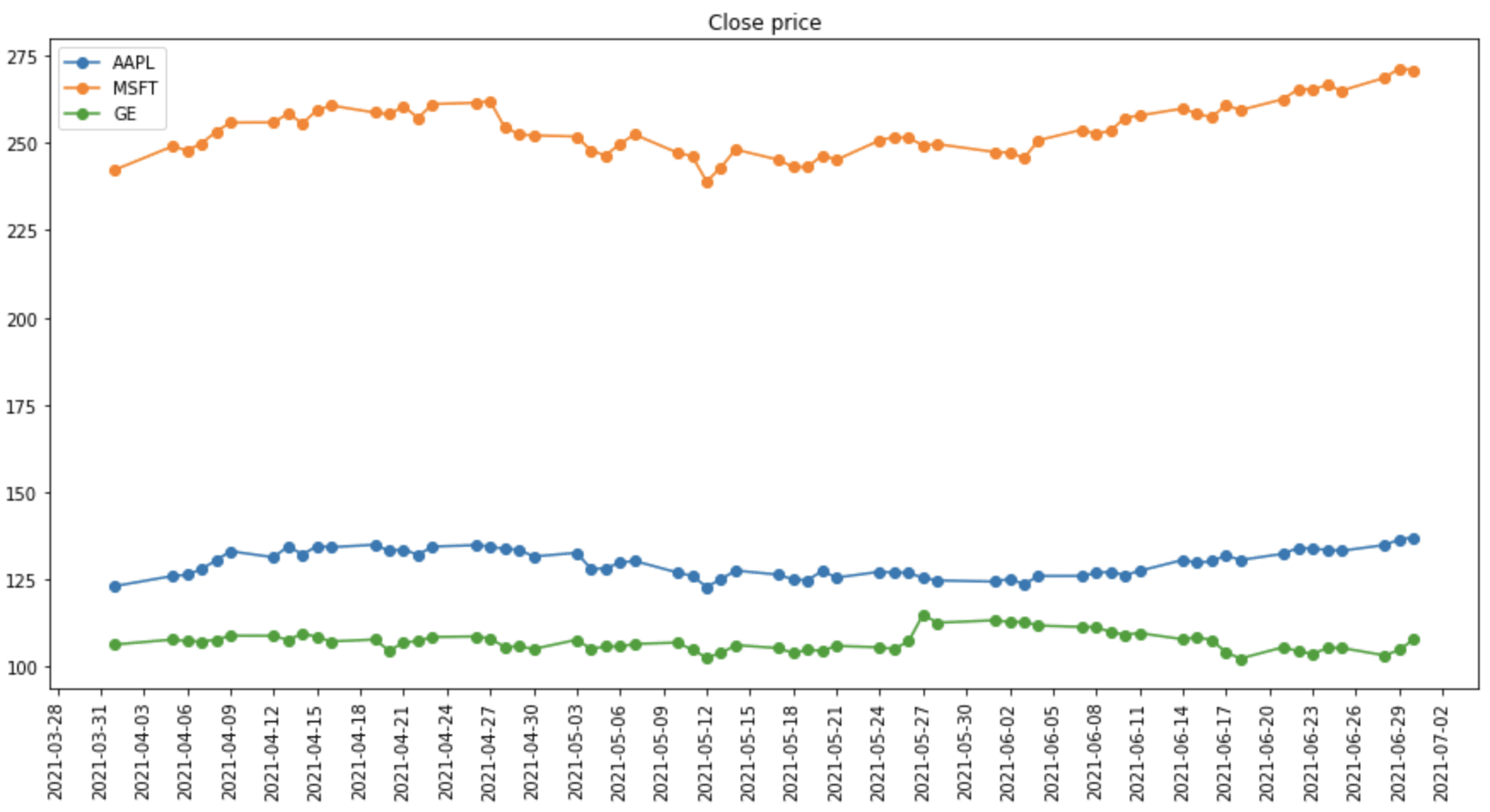
从雅虎财经取来的多只股票
完整的代码如下。
import pandas_datareader as pdr
import matplotlib.pyplot as plt
import matplotlib.ticker as ticker

companies = ['AAPL', 'MSFT', 'GE']
shares_multiple_df = pdr.DataReader(companies, 'yahoo', start='2021-01-01', end='2021-12-31')
print(shares_multiple_df)

def plot_timeseries_df(df, attrib, ticker_loc=1, title='Timeseries', legend=''):
    "General routine for plotting time series data"
    fig = plt.figure(figsize=(15,7))
    plt.plot(df[attrib], 'o-')
    _ = plt.xticks(rotation=90)
    plt.gca().xaxis.set_major_locator(ticker.MultipleLocator(ticker_loc))
    plt.title(title)
    plt.gca().legend(legend)
    plt.show()

plot_timeseries_df(shares_multiple_df.loc["2021-04-01":"2021-06-30"], "Close",
                   ticker_loc=3, title="Close price", legend=companies)
使用pandas-datareader从另一个数据源读取数据的语法是类似的。例如,我们可以从美联储经济数据(FRED)中读取一个经济时间序列。FRED中的每个时间序列都由一个符号来标识。例如,所有城市消费者的消费价格指数是CPIAUCSL,扣除食品和能源的所有项目的消费价格指数是CPILFESL,而个人消费支出是PCE。你可以从FRED的网页上搜索和查询这些符号。
下面是我们如何获得两个消费价格指数,CPIAUCSL和CPILFESL,并在一个图中显示它们。
import pandas_datareader as pdr
import matplotlib.pyplot as plt

# Read data from FRED and print
fred_df = pdr.DataReader(['CPIAUCSL','CPILFESL'], 'fred', "2010-01-01", "2021-12-31")
print(fred_df)

# Show in plot the data of 2019-2021
fig = plt.figure(figsize=(15,7))
plt.plot(fred_df.loc["2019":], 'o-')
plt.xticks(rotation=90)
plt.legend(fred_df.columns)
plt.title("Consumer Price Index")
plt.show()
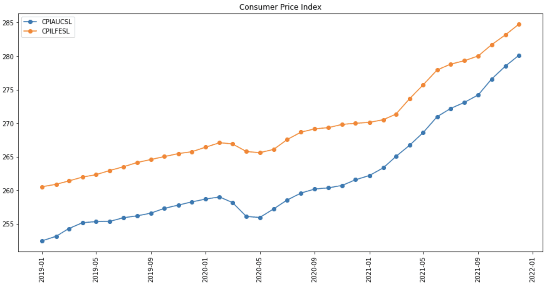
消费者价格指数图
从世界银行获取数据也是类似的,但我们必须明白,世界银行的数据更加复杂。通常,一个数据序列,如人口,是以时间序列的形式呈现的,而且还有国家的维度。因此,我们需要指定更多的参数来获得数据。
使用pandas_datareader ,我们有一套专门针对世界银行的API。一个指标的符号可以从世界银行开放数据中查找,也可以用以下方式搜索。
from pandas_datareader import wb

matches = wb.search('total.*population')
print(matches[["id","name"]])
search() 函数接受一个正则表达式字符串(例如,上面的.* 表示任何长度的字符串)。这将打印。
id                                               name
24     1.1_ACCESS.ELECTRICITY.TOT      Access to electricity (% of total population)
164            2.1_ACCESS.CFT.TOT  Access to Clean Fuels and Technologies for coo...
1999              CC.AVPB.PTPI.AI  Additional people below $1.90 as % of total po...
2000              CC.AVPB.PTPI.AR  Additional people below $1.90 as % of total po...
2001              CC.AVPB.PTPI.DI  Additional people below $1.90 as % of total po...
...                           ...                                                ...
13908           SP.POP.TOTL.FE.ZS         Population, female (% of total population)
13912           SP.POP.TOTL.MA.ZS           Population, male (% of total population)
13938              SP.RUR.TOTL.ZS           Rural population (% of total population)
13958           SP.URB.TOTL.IN.ZS           Urban population (% of total population)
13960              SP.URB.TOTL.ZS  Percentage of Population in Urban Areas (in % ...

[137 rows x 2 columns]
其中id 列是时间序列的符号。
我们可以通过指定ISO-3166-1国家代码来读取特定国家的数据。但是世界银行也包含了非国家的总量(例如南亚),所以虽然pandas_datareader ,允许我们对所有国家使用字符串"all",但通常我们不想使用它。下面是我们如何从世界银行获得所有国家和总量的列表。
import pandas_datareader.wb as wb

countries = wb.get_countries()
print(countries)
iso3c iso2c                 name               region          adminregion          incomeLevel     lendingType capitalCity  longitude  latitude
0     ABW    AW                Aruba  Latin America & ...                               High income  Not classified  Oranjestad   -70.0167   12.5167
1     AFE    ZH  Africa Eastern a...           Aggregates                                Aggregates      Aggregates                    NaN       NaN
2     AFG    AF          Afghanistan           South Asia           South Asia           Low income             IDA       Kabul    69.1761   34.5228
3     AFR    A9               Africa           Aggregates                                Aggregates      Aggregates                    NaN       NaN
4     AFW    ZI  Africa Western a...           Aggregates                                Aggregates      Aggregates                    NaN       NaN
..    ...   ...                  ...                  ...                  ...                  ...             ...         ...        ...       ...
294   XZN    A5  Sub-Saharan Afri...           Aggregates                                Aggregates      Aggregates                    NaN       NaN
295   YEM    YE          Yemen, Rep.  Middle East & No...  Middle East & No...           Low income             IDA      Sana'a    44.2075   15.3520
296   ZAF    ZA         South Africa  Sub-Saharan Africa   Sub-Saharan Afri...  Upper middle income            IBRD    Pretoria    28.1871  -25.7460
297   ZMB    ZM               Zambia  Sub-Saharan Africa   Sub-Saharan Afri...  Lower middle income             IDA      Lusaka    28.2937  -15.3982
298   ZWE    ZW             Zimbabwe  Sub-Saharan Africa   Sub-Saharan Afri...  Lower middle income           Blend      Harare    31.0672  -17.8312
下面是我们如何获得2020年所有国家的人口,并在柱状图中显示前25个国家。当然,我们也可以通过指定不同的start 和end 年来获得跨年度的人口数据。
import pandas_datareader.wb as wb
import pandas as pd
import matplotlib.pyplot as plt

# Get a list of 2-letter country code excluding aggregates
countries = wb.get_countries()
countries = list(countries[countries.region != "Aggregates"]["iso2c"])

# Read countries' total population data (SP.POP.TOTL) in year 2020
population_df = wb.download(indicator="SP.POP.TOTL", country=countries, start=2020, end=2020)

# Sort by population, then take top 25 countries, and make the index (i.e., countries) as a column
population_df = (population_df.dropna()
                              .sort_values("SP.POP.TOTL")
                              .iloc[-25:]
                              .reset_index())

# Plot the population, in millions
fig = plt.figure(figsize=(15,7))
plt.bar(population_df["country"], population_df["SP.POP.TOTL"]/1e6)
plt.xticks(rotation=90)
plt.ylabel("Million Population")
plt.title("Population")
plt.show()
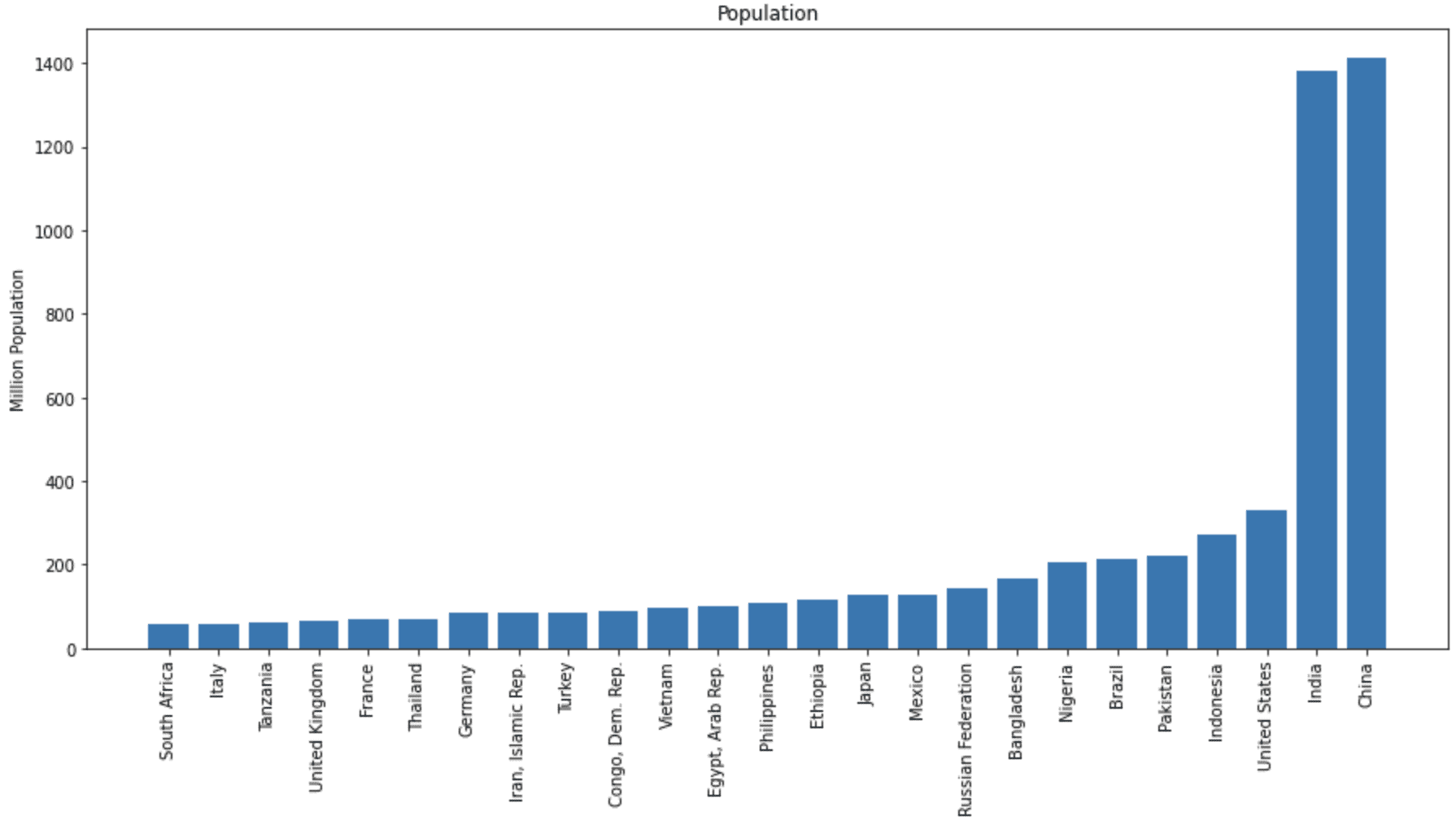
不同国家的总人口条形图
使用Web APIs获取数据
不使用the pandas_datareader 库,有时你可以选择通过调用网络API直接从网络数据服务器获取数据,而不需要任何认证。这可以在Python中使用标准库urllib.requests ,或者你也可以使用requests 库以获得更简单的接口。
世界银行就是一个例子,它的网络API是免费提供的,所以我们可以很容易地读取不同格式的数据,如JSON、XML或纯文本。世界银行数据存储库的API页面描述了各种API和它们各自的参数。为了重复我们在前面的例子中所做的,而不使用pandas_datareader ,我们首先构建一个URL来读取所有国家的列表,这样我们就可以找到不是聚合的国家代码。然后,我们可以用以下参数构建一个查询URL。
country参数的值 =allindicator参数值=SP.POP.TOTLdate参数值=2020format参数值=json
当然,你可以尝试使用不同的指标。默认情况下,世界银行在一个页面上返回50个项目,我们需要一个又一个页面的查询来耗尽数据。我们可以放大页面大小,一次性获得所有数据。下面是我们如何获得JSON格式的国家列表并收集国家代码。
import requests

# Create query URL for list of countries, by default only 50 entries returned per page
url = "http://api.worldbank.org/v2/country/all?format=json&per_page=500"
response = requests.get(url)
# Expects HTTP status code 200 for correct query
print(response.status_code)
# Get the response in JSON
header, data = response.json()
print(header)
# Collect a list of 3-letter country code excluding aggregates
countries = [item["id"]
             for item in data
             if item["region"]["value"] != "Aggregates"]
print(countries)
它将打印出HTTP状态代码、标题和国家代码列表,如下所示。
200
{'page': 1, 'pages': 1, 'per_page': '500', 'total': 299}
['ABW', 'AFG', 'AGO', 'ALB', ..., 'YEM', 'ZAF', 'ZMB', 'ZWE']
从标题中,我们可以验证我们用尽了数据(第1页,共1页)。然后我们可以得到所有的人口数据,如下所示。
...

# Create query URL for total population from all countries in 2020
arguments = {
    "country": "all",
    "indicator": "SP.POP.TOTL",
    "date": "2020:2020",
    "format": "json"
}
url = "http://api.worldbank.org/v2/country/{country}/" \
      "indicator/{indicator}?date={date}&format={format}&per_page=500"
query_population = url.format(**arguments)
response = requests.get(query_population)
# Get the response in JSON
header, population_data = response.json()
你应该查看世界银行的API文档,了解如何构建URL的细节。例如,2020:2021 的日期语法将意味着开始和结束的年份,而额外的参数page=3 将给你多页结果中的第三页。拿到数据后,我们可以只过滤那些非综合国家,把它做成一个pandas DataFrame进行排序,然后绘制柱状图。
...

# Filter for countries, not aggregates
population = []
for item in population_data:
    if item["countryiso3code"] in countries:
        name = item["country"]["value"]
        population.append({"country":name, "population": item["value"]})
# Create DataFrame for sorting and filtering
population = pd.DataFrame.from_dict(population)
population = population.dropna().sort_values("population").iloc[-25:]
# Plot bar chart
fig = plt.figure(figsize=(15,7))
plt.bar(population["country"], population["population"]/1e6)
plt.xticks(rotation=90)
plt.ylabel("Million Population")
plt.title("Population")
plt.show()
图中的内容应该和之前的完全一样。但正如你所看到的,使用pandas_datareader ,通过隐藏低级别的操作,有助于使代码更加简洁。
把所有东西放在一起,下面是完整的代码。
import pandas as pd
import matplotlib.pyplot as plt
import requests


# Create query URL for list of countries, by default only 50 entries returned per page
url = "http://api.worldbank.org/v2/country/all?format=json&per_page=500"
response = requests.get(url)
# Expects HTTP status code 200 for correct query
print(response.status_code)
# Get the response in JSON
header, data = response.json()
print(header)
# Collect a list of 3-letter country code excluding aggregates
countries = [item["id"]
             for item in data
             if item["region"]["value"] != "Aggregates"]
print(countries)


# Create query URL for total population from all countries in 2020
arguments = {
    "country": "all",
    "indicator": "SP.POP.TOTL",
    "date": 2020,
    "format": "json"
}
url = "http://api.worldbank.org/v2/country/{country}/" \
      "indicator/{indicator}?date={date}&format={format}&per_page=500"
query_population = url.format(**arguments)
response = requests.get(query_population)
print(response.status_code)
# Get the response in JSON
header, population_data = response.json()
print(header)


# Filter for countries, not aggregates
population = []
for item in population_data:
    if item["countryiso3code"] in countries:
        name = item["country"]["value"]
        population.append({"country":name, "population": item["value"]})
# Create DataFrame for sorting and filtering
population = pd.DataFrame.from_dict(population)
population = population.dropna().sort_values("population").iloc[-25:]
# Plot bar chart
fig = plt.figure(figsize=(15,7))
plt.bar(population["country"], population["population"]/1e6)
plt.xticks(rotation=90)
plt.ylabel("Million Population")
plt.title("Population")
plt.show()
使用NumPy创建合成数据
有时,我们可能不想在我们的项目中使用真实世界的数据,因为我们需要一些在现实中可能不会发生的特殊情况。一个特别的例子是用理想的时间序列数据来测试一个模型。在本节中,我们将看到如何创建合成自回归(AR)时间序列数据。
numpy.random库可以用来创建来自不同分布的随机样本。randn() 方法从具有零平均数和单位方差的标准正态分布中生成数据。
在阶数为的AR()模型中,时间步数的值取决于之前时间步数的值。就是说。
模型参数为不同滞后期的系数,误差项预计将遵循正态分布。
了解了这个公式,我们就可以在下面的例子中生成一个AR(3)时间序列。我们首先使用randn() 来生成序列的前3个值,然后迭代应用上述公式来生成下一个数据点。然后,再次使用the randn() 函数添加一个误差项,但要符合预定义的noise_level 。
import numpy as np

# Predefined paramters
ar_n = 3                     # Order of the AR(n) data
ar_coeff = [0.7, -0.3, -0.1] # Coefficients b_3, b_2, b_1
noise_level = 0.1            # Noise added to the AR(n) data
length = 200                 # Number of data points to generate

# Random initial values
ar_data = list(np.random.randn(ar_n))

# Generate the rest of the values
for i in range(length - ar_n):
    next_val = (np.array(ar_coeff) @ np.array(ar_data[-3:])) + np.random.randn() * noise_level
    ar_data.append(next_val)

# Plot the time series
fig = plt.figure(figsize=(12,5))
plt.plot(ar_data)
plt.show()
上面的代码将创建以下图表:

但我们可以进一步添加时间轴,首先将数据转换为pandas DataFrame,然后添加时间作为索引。
...

# Convert the data into a pandas DataFrame
synthetic = pd.DataFrame({"AR(3)": ar_data})
synthetic.index = pd.date_range(start="2021-07-01", periods=len(ar_data), freq="D")

# Plot the time series
fig = plt.figure(figsize=(12,5))
plt.plot(synthetic.index, synthetic)
plt.xticks(rotation=90)
plt.title("AR(3) time series")
plt.show()
之后,我们就会有下面的图了。
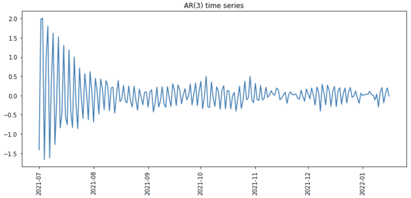
合成时间序列的图
使用类似的技术,我们也可以生成纯随机噪声(即AR(0)序列)、ARIMA时间序列(即有系数的误差项)或布朗运动时间序列(即随机噪声的运行和)。
摘要
在本教程中,你发现了在Python中获取数据或生成合成时间序列数据的各种选项。
具体来说,你学到了
- 如何使用
pandas_datareader,从不同的数据源获取金融数据 - 如何使用
the requests库调用API从不同的网络服务器获取数据 - 如何使用NumPy的随机数发生器生成合成时间序列数据
