本文已参与「新人创作礼」活动，一起开启掘金创作之路。

softmax

为了让自己的cs231n学习更加高效且容易复习，特此在这里记录学习过程，以供参考。

作用机理

softmax其实和SVM差别不大，两者损失函数不同，softmax就是把各个类的得分转化成了概率，因此所有类的概率加在一起等于1。 softmax函数：

S_i=\frac{e^{S_{y_i}}}{\sum^C_{j=1}e^{S_j}}

softmax的输入：

L_i=-S_i=-log\frac{e^{S_{y_i}}}{\sum^C_{j=1}e^{S_j}}

它的等价形式：

L_i=-log\frac{e^{S_{y_i}}}{\sum^C_{j=1}e^{S_j}}=-(s_{y_i}-log\sum_{j=1}^Ce^{s_j})=-s_{y_i}+log\sum_{j=1}^C e^{s_j}

同时要注意数值爆炸问题（blog.csdn.net/Sean_csy/ar…

在实际使用中，常常因为指数太大而出现数值爆炸问题，两个非常大的数相除会出现数值不稳定问题，因此我们需要在分子和分母中同时进行以下处理：

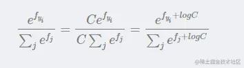
其中C 的设置是任意的，在实际变成中，往往把C设置成：

即第 i个样本所有分值中最大的值，当现有分值减去该最大分值后结果≤0，放在 e 的指数上可以保证分子分布都在0-1之内

梯度推导：在这里插入图片描述

Assignment 1的softmax作业

下面我们进入代码编辑

softmax.ipynb(1)

Softmax exercise
Complete and hand in this completed worksheet (including its outputs and any supporting code outside of the worksheet) with your assignment submission. For more details see the assignments page on the course website.

This exercise is analogous to the SVM exercise. You will:

1.implement a fully-vectorized loss function for the Softmax classifier
2.implement the fully-vectorized expression for its analytic gradient
3.check your implementation with numerical gradient
4.use a validation setto tune the learning rate and regularization strength optimize the loss function with SGD
5.visualize the final learned weights\

练习目的：
1.为softmax分类器实现完全矢量化的损失函数
2.实现其解析梯度的全矢量表达式
3.用数值梯度检查您的实现
4.使用验证设置来调整学习速率和正则化强度，使用SGD优化损失函数
5.可视化最终学习的权重

import random
import numpy as np
from cs231n.data_utils import load_CIFAR10
import matplotlib.pyplot as plt

%matplotlib inline
plt.rcParams['figure.figsize'] = (10.0, 8.0) # set default size of plots
plt.rcParams['image.interpolation'] = 'nearest'
plt.rcParams['image.cmap'] = 'gray'

# for auto-reloading extenrnal modules
# see http://stackoverflow.com/questions/1907993/autoreload-of-modules-in-ipython
%load_ext autoreload
%autoreload 2

设置初始参数，图像大小等等。

def get_CIFAR10_data(num_training=49000, num_validation=1000, num_test=1000, num_dev=500):
    """
    Load the CIFAR-10 dataset from disk and perform preprocessing to prepare
    it for the linear classifier. These are the same steps as we used for the
    SVM, but condensed to a single function.  
    """
    # Load the raw CIFAR-10 data
    cifar10_dir = 'cs231n/datasets/cifar-10-batches-py'
    
    # Cleaning up variables to prevent loading data multiple times (which may cause memory issue)
    try:
       del X_train, y_train
       del X_test, y_test
       print('Clear previously loaded data.')
    except:
       pass

    X_train, y_train, X_test, y_test = load_CIFAR10(cifar10_dir)
    
    # subsample the data
    mask = list(range(num_training, num_training + num_validation)) #验证集
    X_val = X_train[mask]
    y_val = y_train[mask]
    mask = list(range(num_training)) #训练集
    X_train = X_train[mask]
    y_train = y_train[mask]
    mask = list(range(num_test)) #测试集
    X_test = X_test[mask]
    y_test = y_test[mask]
    mask = np.random.choice(num_training, num_dev, replace=False) #随机集
    X_dev = X_train[mask]
    y_dev = y_train[mask]
    
    # Preprocessing: reshape the image data into rows （打乱顺序）
    X_train = np.reshape(X_train, (X_train.shape[0], -1))
    X_val = np.reshape(X_val, (X_val.shape[0], -1))
    X_test = np.reshape(X_test, (X_test.shape[0], -1))
    X_dev = np.reshape(X_dev, (X_dev.shape[0], -1))
    
    # Normalize the data: subtract the mean image （归一化）
    mean_image = np.mean(X_train, axis = 0)
    X_train -= mean_image
    X_val -= mean_image
    X_test -= mean_image
    X_dev -= mean_image
    
    # add bias dimension and transform into columns （添加偏执）
    X_train = np.hstack([X_train, np.ones((X_train.shape[0], 1))])
    X_val = np.hstack([X_val, np.ones((X_val.shape[0], 1))])
    X_test = np.hstack([X_test, np.ones((X_test.shape[0], 1))])
    X_dev = np.hstack([X_dev, np.ones((X_dev.shape[0], 1))])
    
    return X_train, y_train, X_val, y_val, X_test, y_test, X_dev, y_dev


# Invoke the above function to get our data.
X_train, y_train, X_val, y_val, X_test, y_test, X_dev, y_dev = get_CIFAR10_data()
print('Train data shape: ', X_train.shape)
print('Train labels shape: ', y_train.shape)
print('Validation data shape: ', X_val.shape)
print('Validation labels shape: ', y_val.shape)
print('Test data shape: ', X_test.shape)
print('Test labels shape: ', y_test.shape)
print('dev data shape: ', X_dev.shape)
print('dev labels shape: ', y_dev.shape)

↑具体作用见代码注释，下面是结果：

Train data shape: (49000, 3073)
Train labels shape: (49000,)
Validation data shape: (1000, 3073)
Validation labels shape: (1000,)
Test data shape: (1000, 3073)
Test labels shape: (1000,)
dev data shape: (500, 3073)
dev labels shape: (500,)

下面进入softmax.py完成作业

Softmax Classifier
Your code for this section will all be written inside cs231n/classifiers/softmax.py.

softmax.py

from builtins import range
import numpy as np
from random import shuffle
from past.builtins import xrange

def softmax_loss_naive(W, X, y, reg):
    """
    Softmax loss function, naive implementation (with loops)

    Inputs have dimension D, there are C classes, and we operate on minibatches
    of N examples.

    Inputs:
    - W: A numpy array of shape (D, C) containing weights.
    - X: A numpy array of shape (N, D) containing a minibatch of data.
    - y: A numpy array of shape (N,) containing training labels; y[i] = c means
      that X[i] has label c, where 0 <= c < C.
    - reg: (float) regularization strength

    Returns a tuple of:
    - loss as single float
    - gradient with respect to weights W; an array of same shape as W
    """
    # Initialize the loss and gradient to zero.
    loss = 0.0
    dW = np.zeros_like(W)

    #############################################################################
    # TODO: Compute the softmax loss and its gradient using explicit loops.     #
    # Store the loss in loss and the gradient in dW. If you are not careful     #
    # here, it is easy to run into numeric instability. Don't forget the        #
    # regularization!                                                           #
    #############################################################################
    # *****START OF YOUR CODE (DO NOT DELETE/MODIFY THIS LINE)*****

    num_classes = W.shape[1]
    num_train = X.shape[0]
    for i in range(num_train):
        scores = np.dot(X[i], W)
        scores -= np.max(scores)
        correct_class_score = scores[y[i]]
        exp_sum = np.sum(np.exp(scores))
        loss += -correct_class_score + np.log(exp_sum) # 公式
        for j in range(num_classes):
            if j == y[i]:
                dW[:, j] += X[i] * (-1+(np.exp(scores[j]) / exp_sum))  #dL/dW=(Pk-1(Yi=k))*x
            else:
                dW[:, j] += X[i] * (np.exp(scores[j]) / exp_sum)


    loss /= num_train
    loss += 0.5 * reg * np.sum(W * W)
    dW /= num_train
    dW += reg * W

    pass

    # *****END OF YOUR CODE (DO NOT DELETE/MODIFY THIS LINE)*****

    return loss, dW


def softmax_loss_vectorized(W, X, y, reg):
    """
    Softmax loss function, vectorized version.

    Inputs and outputs are the same as softmax_loss_naive.
    """
    # Initialize the loss and gradient to zero.
    loss = 0.0
    dW = np.zeros_like(W)

    #############################################################################
    # TODO: Compute the softmax loss and its gradient using no explicit loops.  #
    # Store the loss in loss and the gradient in dW. If you are not careful     #
    # here, it is easy to run into numeric instability. Don't forget the        #
    # regularization!                                                           #
    #############################################################################
    # *****START OF YOUR CODE (DO NOT DELETE/MODIFY THIS LINE)*****

    num_classes = W.shape[1]
    num_train = X.shape[0]

    scores = np.dot(X, W)
    #print(scores.shape) #(500,10)
    scores -= np.max(scores, axis=1,keepdims=True)  # 减去最大值防爆数
    #print(scores.shape) #(500,)
    #print(scores[range(num_train), y].shape) # (500,) 一维
    #print(y.shape) (500,)
    correct_class_scores = np.sum(scores[range(num_train), y]) #这句不怎么懂。

    scores = np.exp(scores)
    exp_sum = np.sum(scores, axis=1, keepdims=True) #往y轴上投影
    #print(exp_sum.shape) #(500,1)

    loss = -correct_class_scores + np.sum(np.log(exp_sum)) #公式 L=-Si+log()
    loss = loss / num_train + 0.5 * reg * np.sum(W * W)


    #根据公式 softmax求导的公式，分类讨论。

    prob = scores / exp_sum
    #print(prob.shape) #（500，10）
    prob[range(num_train), y] -= 1    #把 -Xi 项“分配”进梯度的公式里 因为j=Yi时候，dW的结果有一项-Xi

    #print(X.shape) #(500, 3073)
    dW = np.dot(X.T, prob)
    dW = dW / num_train + reg * W

    pass

    # *****END OF YOUR CODE (DO NOT DELETE/MODIFY THIS LINE)*****

    return loss, dW

↑相关注释已经写在代码里了

softmax.py(2)

接下来我们回到softmax.py

# First implement the naive softmax loss function with nested loops.
# Open the file cs231n/classifiers/softmax.py and implement the
# softmax_loss_naive function.

from cs231n.classifiers.softmax import softmax_loss_naive
import time

# Generate a random softmax weight matrix and use it to compute the loss.
W = np.random.randn(3073, 10) * 0.0001
loss, grad = softmax_loss_naive(W, X_dev, y_dev, 0.0)

# As a rough sanity check, our loss should be something close to -log(0.1).
print('loss: %f' % loss)
print('sanity check: %f' % (-np.log(0.1)))

↑随机选择权重并计算loss，检查loss值是否合理：

loss: 2.377748
sanity check: 2.302585

这里有一个小问题：

Inline Question 1
Why do we expect our loss to be close to -log(0.1)? Explain briefly.**
Y𝑜𝑢𝑟𝐴𝑛𝑠𝑤𝑒𝑟: Fill this in

问的就是有关loss值检查的问题，我们的loss为什么应该近似等于-log(0.1)

# Complete the implementation of softmax_loss_naive and implement a (naive)
# version of the gradient that uses nested loops.
loss, grad = softmax_loss_naive(W, X_dev, y_dev, 0.0)

# As we did for the SVM, use numeric gradient checking as a debugging tool.
# The numeric gradient should be close to the analytic gradient.
from cs231n.gradient_check import grad_check_sparse
f = lambda w: softmax_loss_naive(w, X_dev, y_dev, 0.0)[0]
grad_numerical = grad_check_sparse(f, W, grad, 10)

# similar to SVM case, do another gradient check with regularization
loss, grad = softmax_loss_naive(W, X_dev, y_dev, 5e1)
f = lambda w: softmax_loss_naive(w, X_dev, y_dev, 5e1)[0]
grad_numerical = grad_check_sparse(f, W, grad, 10)

↑梯度检查

numerical: 0.991854 analytic: 0.991854, relative error: 3.737526e-08
numerical: -0.532129 analytic: -0.532129, relative error: 9.010182e-08
numerical: -0.860263 analytic: -0.860263, relative error: 1.652241e-08
numerical: 0.231419 analytic: 0.231419, relative error: 1.820207e-08
numerical: 0.638393 analytic: 0.638393, relative error: 4.364700e-08
numerical: 1.454550 analytic: 1.454550, relative error: 6.796846e-09
numerical: -0.150960 analytic: -0.150960, relative error: 1.317062e-07
numerical: 1.199503 analytic: 1.199503, relative error: 3.188985e-08
numerical: 1.097738 analytic: 1.097738, relative error: 1.216716e-08
numerical: 0.643756 analytic: 0.643756, relative error: 1.885507e-09
numerical: -1.743187 analytic: -1.743187, relative error: 1.394700e-08
numerical: -0.039634 analytic: -0.039634, relative error: 6.152723e-07
numerical: -1.221929 analytic: -1.221929, relative error: 1.063883e-08
numerical: -2.243449 analytic: -2.243449, relative error: 2.059132e-08
numerical: -0.873285 analytic: -0.873285, relative error: 5.913211e-08
numerical: -3.040440 analytic: -3.040440, relative error: 3.536497e-09
numerical: -2.229787 analytic: -2.229787, relative error: 1.154475e-08
numerical: 0.034711 analytic: 0.034711, relative error: 9.975545e-08
numerical: 1.338736 analytic: 1.338736, relative error: 1.417860e-09
numerical: 0.863464 analytic: 0.863464, relative error: 8.883882e-09

# Now that we have a naive implementation of the softmax loss function and its gradient,
# implement a vectorized version in softmax_loss_vectorized.
# The two versions should compute the same results, but the vectorized version should be
# much faster.
tic = time.time()
loss_naive, grad_naive = softmax_loss_naive(W, X_dev, y_dev, 0.000005)
toc = time.time()
print('naive loss: %e computed in %fs' % (loss_naive, toc - tic))

from cs231n.classifiers.softmax import softmax_loss_vectorized
tic = time.time()
loss_vectorized, grad_vectorized = softmax_loss_vectorized(W, X_dev, y_dev, 0.000005)
toc = time.time()
print('vectorized loss: %e computed in %fs' % (loss_vectorized, toc - tic))

# As we did for the SVM, we use the Frobenius norm to compare the two versions
# of the gradient.
grad_difference = np.linalg.norm(grad_naive - grad_vectorized, ord='fro')
print('Loss difference: %f' % np.abs(loss_naive - loss_vectorized))
print('Gradient difference: %f' % grad_difference)

↑计算naive loss和vectorized loss，评估运算时间：

naive loss: 2.377748e+00 computed in 0.135166s
vectorized loss: 2.377748e+00 computed in 0.180172s
Loss difference: 0.000000
Gradient difference: 0.000000

# Use the validation set to tune hyperparameters (regularization strength and
# learning rate). You should experiment with different ranges for the learning
# rates and regularization strengths; if you are careful you should be able to
# get a classification accuracy of over 0.35 on the validation set.

from cs231n.classifiers import Softmax
results = {}
best_val = -1
best_softmax = None

################################################################################
# TODO:                                                                        #
# Use the validation set to set the learning rate and regularization strength. #
# This should be identical to the validation that you did for the SVM; save    #
# the best trained softmax classifer in best_softmax.                          #
################################################################################

# Provided as a reference. You may or may not want to change these hyperparameters
learning_rates = [1e-7, 5e-7]
regularization_strengths = [2.5e4, 5e4]

# *****START OF YOUR CODE (DO NOT DELETE/MODIFY THIS LINE)*****

for lr in learning_rates:
    for rs in regularization_strengths:
        softmax = Softmax()
        softmax.train(X_train, y_train, lr, rs, num_iters=2000)
        y_train_pred = softmax.predict(X_train)
        train_accuracy = np.mean(y_train == y_train_pred)
        y_val_pred = softmax.predict(X_val)
        val_accuracy = np.mean(y_val == y_val_pred)
        if val_accuracy > best_val:
            best_val = val_accuracy
            best_softmax = softmax           
        results[(lr,rs)] = train_accuracy, val_accuracy
pass

# *****END OF YOUR CODE (DO NOT DELETE/MODIFY THIS LINE)*****
    
# Print out results.
for lr, reg in sorted(results):
    train_accuracy, val_accuracy = results[(lr, reg)]
    print('lr %e reg %e train accuracy: %f val accuracy: %f' % (
                lr, reg, train_accuracy, val_accuracy))
    
print('best validation accuracy achieved during cross-validation: %f' % best_val)

↑选择合适的正则化参数和学习率：

lr 1.000000e-07 reg 2.500000e+04 train accuracy: 0.350857 val accuracy: 0.370000 lr 1.000000e-07 reg 5.000000e+04 train accuracy: 0.330490 val accuracy: 0.343000 lr 5.000000e-07 reg 2.500000e+04 train accuracy: 0.346592 val accuracy: 0.356000 lr 5.000000e-07 reg 5.000000e+04 train accuracy: 0.330796 val accuracy: 0.340000 best validation accuracy achieved during cross-validation: 0.370000

# evaluate on test set
# Evaluate the best softmax on test set
y_test_pred = best_softmax.predict(X_test)
test_accuracy = np.mean(y_test == y_test_pred)
print('softmax on raw pixels final test set accuracy: %f' % (test_accuracy, ))

测试集跑一下，得到准确率：

softmax on raw pixels final test set accuracy: 0.351000

Inline Question 2 - True or False
Suppose the overall training loss is defined as the sum of the per-datapoint loss over all training examples. It is possible to add a new datapoint to a training set that would leave the SVM loss unchanged, but this is not the case with the Softmax classifier loss.
Y𝑜𝑢𝑟𝐴𝑛𝑠𝑤𝑒𝑟:
Y𝑜𝑢𝑟𝐸𝑥𝑝𝑙𝑎𝑛𝑎𝑡𝑖𝑜𝑛:

这里是第二个小问题，假设总的训练损失被定义为所有训练示例中每个数据点损失的总和。可以向训练集中添加一个新的数据点，使svm损失保持不变，但softmax分类器的损失不会保持不变。这句陈述正确吗？我认为是正确的，对于SVM分类器，这个数据点可能最后取值为0；而对于softmax，得到的是一个概率，因此loss一定会增加。

# Visualize the learned weights for each class
w = best_softmax.W[:-1,:] # strip out the bias
w = w.reshape(32, 32, 3, 10)

w_min, w_max = np.min(w), np.max(w)

classes = ['plane', 'car', 'bird', 'cat', 'deer', 'dog', 'frog', 'horse', 'ship', 'truck']
for i in range(10):
    plt.subplot(2, 5, i + 1)
    
    # Rescale the weights to be between 0 and 255
    wimg = 255.0 * (w[:, :, :, i].squeeze() - w_min) / (w_max - w_min)
    plt.imshow(wimg.astype('uint8'))
    plt.axis('off')
    plt.title(classes[i])

↑最后是可视化：在这里插入图片描述

Softmax及cs231n作业解读