对服装图像进行分类

import tensorflow as tf 
from tensorflow import keras
import numpy as np
import matplotlib.pyplot as plt

1. 导入 fashion MNIST 数据集

fashion_nmist = keras.datasets.fashion_mnist
(train_image,train_labels),(test_images,test_labels) = fashion_nmist.load_data()

Fashion MNIST是临时替代 MNIST 的数据集，后者具有经典的手写数字等图像。

数据加载完毕会返回 4 个 numpy 数组：

train_image,train_labels为训练集，用于学习的数据 - test_images,test_labels 为测试集，用来对模型进行预测其中，每张图片都是 28*28 的 numpy 数组，像素基于 0-25 之间，标签为整数数组，0-9 之间，每个标签对应不同的服装类：

# 列表索引编号与标签对应
class_names = ['T-shirt/top', 'Trouser', 'Pullover', 'Dress', 'Coat', 'Sandal', 'Shirt', 'Sneaker', 'Bag', 'Ankle boot']

2. 浏览数据

训练集

train_image.shape
train_labels.shape #len(train.labels)

测试集

test_images.shape
len(test_labels)

3. 预处理数据

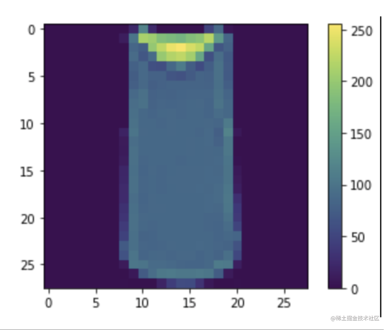
查看其中一个图像

plt.figure()
plt.imshow(train_image[2])
plt.colorbar()
plt.grid(False)
plt.show()

结果如下

将所有的值压缩在 0-1 之间，将其馈送到神经模型网络，训练集和测试集全部除以 255，然后进行验证。

train_image = train_image/255
test_images = test_images/255

![image.png](https://p1-juejin.byteimg.com/tos-cn-i-k3u1fbpfcp/7bc5d19e4eec497197ac6fc0138b92ca~tplv-k3u1fbpfcp-watermark.image?)
plt.figure(figsize = (10,10))
for i in range(25):
    plt.subplot(5,5,i+1)
    plt.xticks([])
    plt.yticks([])
    plt.grid(False)
    plt.imshow(train_image[i],cmap= plt.cm.binary)
    plt.xlabel(class_names[train_labels[I]])
plt.show()

4. 构建模型

构建神经网络需要先配置模型的层，然后在编译模型。

4.1 设置层

model = keras.Sequential([
    keras.layers.Flatten(input_shape=(28,28)),
    keras.layers.Dense(128,activation = 'relu'),
    keras.layers.Dense(10)
])

神经网络的基本结构是层，

该网络的第一层是将图像从二维数组（2828 像素）转换成一维数组（2828 =784 像素）（展平像素）

展平像素后，网络会包括两个 keras.layers.Dense层的序列。他们是密集连接或全连接神经层，第一个层有 128 个节点（神经元），第二个层会返回一个长度为 1- 的 logits 数组。

每个节点都包含一个得分，用来标示当前图像属于 10 个类中的那个

4.2 编译模型

model.compile(optimizer = 'Adam',
             loss = tf.keras.losses.SparseCategoricalCrossentropy(from_logits=True),
             metrics=['accuracy'])

优化器：决定模型如何根据其看到的数据和自身的损失函数进行更新

损失函数：用于测量模型在虚拟兰期间的准确率

指标：用于监控训练和测试步骤，accuracy 代表的是准确率。

5. 训练模型

训练模型的步骤

将训练数据馈送给模型。在本例中，训练数据位于 train_images 和 train_labels 数组中。
模型学习将图像和标签关联起来。
要求模型对测试集（在本例中为 test_images 数组）进行预测。
验证预测是否与 test_labels 数组中的标签相匹配。

5.1 向模型馈送数据

model.fit(train_image,train_labels,epochs = 10)

在训练模型期间，会显示损失和准确率的指标。

5.2 评估准确率

test_loss,test_acc = model.evaluate(test_images,test_labels,verbose=2)
print('\n Test accuract:',test_acc)

结果表明，模型在测试数据集上的准确率略低于训练数据集。训练准确率和测试准确率之间的差距代表过拟合。过拟合是指机器学习模型在新的、以前未曾见过的输入上的表现不如在训练数据上的表现。过拟合的模型会“记住”训练数据集中的噪声和细节，从而对模型在新数据上的表现产生负面影响。有关更多信息，请参阅以下内容：

5.3 进行预测

模型经过训练后，还可以使用它对图像进行预测。模型具有线性输出，即logits，我们可以加一个 softmax，将 logits 转换成更加容易理解的。

predictions = probability_model.predict(test_images)
predictions[0]

np.argmax(predictions[0])

预测结果是一个包含 10 个数字的数组。它们代表模型对 10 种不同服装中每种服装的“置信度”。您可以看到哪个标签的置信度值最大

通过绘制成图图表，查看模型对于所有 10 个类的预测。

def plot_image(i, predictions_array, true_label, img):
  predictions_array, true_label, img = predictions_array, true_label[i], img[I]
  plt.grid(False)
  plt.xticks([])
  plt.yticks([])

  plt.imshow(img, cmap=plt.cm.binary)

  predicted_label = np.argmax(predictions_array)
  if predicted_label == true_label:
    color = 'blue'
  else:
    color = 'red'

  plt.xlabel("{} {:2.0f}% ({})".format(class_names[predicted_label],
                                100*np.max(predictions_array),
                                class_names[true_label]),
                                color=color)

def plot_value_array(i, predictions_array, true_label):
  predictions_array, true_label = predictions_array, true_label[I]
  plt.grid(False)
  plt.xticks(range(10))
  plt.yticks([])
  thisplot = plt.bar(range(10), predictions_array, color="#777777")
  plt.ylim([0, 1])
  predicted_label = np.argmax(predictions_array)

  thisplot[predicted_label].set_color('red')
  thisplot[true_label].set_color('blue')

5.4 验证预测结果

在模型经过训练后，您可以使用它对一些图像进行预测。

我们来看看第 0 个图像、预测结果和预测数组。正确的预测标签为蓝色，错误的预测标签为红色。数字表示预测标签的百分比（总计为 100）。

i = 0
plt.figure(figsize=(6,3))
plt.subplot(1,2,1)
plot_image(i, predictions[i], test_labels, test_images)
plt.subplot(1,2,2)
plot_value_array(i, predictions[i],  test_labels)
plt.show()

让我们用模型的预测绘制几张图像。请注意，即使置信度很高，模型也可能出错。

# Plot the first X test images, their predicted labels, and the true labels.
# Color correct predictions in blue and incorrect predictions in red.
num_rows = 5
num_cols = 3
num_images = num_rows*num_cols
plt.figure(figsize=(2*2*num_cols, 2*num_rows))
for i in range(num_images):
  plt.subplot(num_rows, 2*num_cols, 2*I+1)
  plot_image(i, predictions[i], test_labels, test_images)
  plt.subplot(num_rows, 2*num_cols, 2*I+2)
  plot_value_array(i, predictions[i], test_labels)
plt.tight_layout()
plt.show()

使用训练好的模型

对一个样本进行预测

img = test_images[1]
img.shape #(28,28)

当批量预测时，即使只有一个样本，也必须将其添加到列表中：

img =(np.expand_dims(img,0))
img.shape  # (1,28,28)

然后对这个图像进行标签预测：

predictions_single = probability_model(img)
print(predictions_single）

画图

plot_value_array(1, predictions_single[0], test_labels)
_ = plt.xticks(range(10), class_names, rotation=45)

keras.Model.predict 会返回一组列表，每个列表对应一批数据中的每个图像。在批次中获取对我们（唯一）图像的预测

np.argmax(predictions_single[0])

TensorFlow教程汇总--Keras 机器学习基础① 对服装图像进行分类