计算视觉——图像的局部特征信息及全景图像拼接

1 背景

理论中对图像的处理通常分为三种，与一些简单的计算相关的低层视觉（图像统计与简单计算，如直方图、滤波、纹理等），与一些已知人眼视觉特性相关的中层视觉（图像理解，如梯度、匹配跟踪、图像特征等），与人眼视觉特性、思维方式高度相关的高级视觉（图像理解，如分类、检测、基于语义的处理等）。

其中，图像特征是一种老生常谈的图像信息，早期的方法如梯度提取算子、图像的局部直方图等都可以作为图像的局部特征去使用。而近年来被广泛关注的卷积神经网络等方法，也是通过卷积等网络框架去得到一层（或多层）特定大小的特征图，以此作为图像的特征，实现分类等特定的目的。

本文将聚焦于传统图像处理中的局部特征计算，并介绍一种图像局部特征的应用——全景图像拼接。

2 局部特征提取中存在的问题

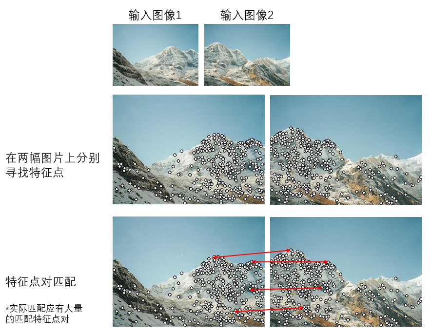
图像特征信息是图像中的重要信息，在图像匹配、图像拼接等方面有不可替代的作用，如果不利用图像特征，我们几乎找不出其他行之有效的方法去解决图像匹配等问题，如下图所示。

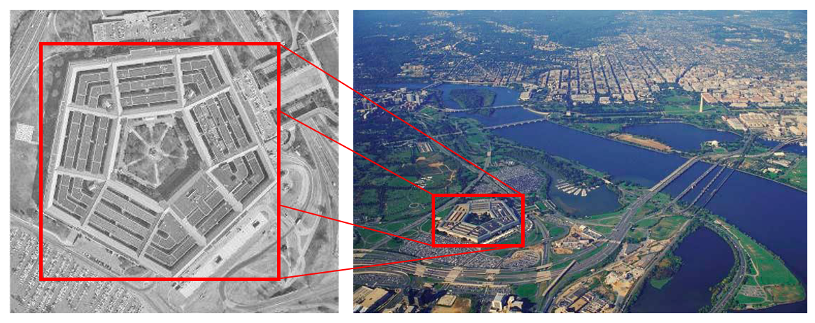
通过直接的视觉判别，我们很容易匹配出两幅图像相同的地方，但是如何让计算机自动、流程化地区实现图像匹配，这就需要提取图像的特征并实现匹配。

但是图像的特征信息并不是那么容易就可以得到的，如果不参考相关的研究自己琢磨怎么去提取特征，那么迎面而来的问题如下

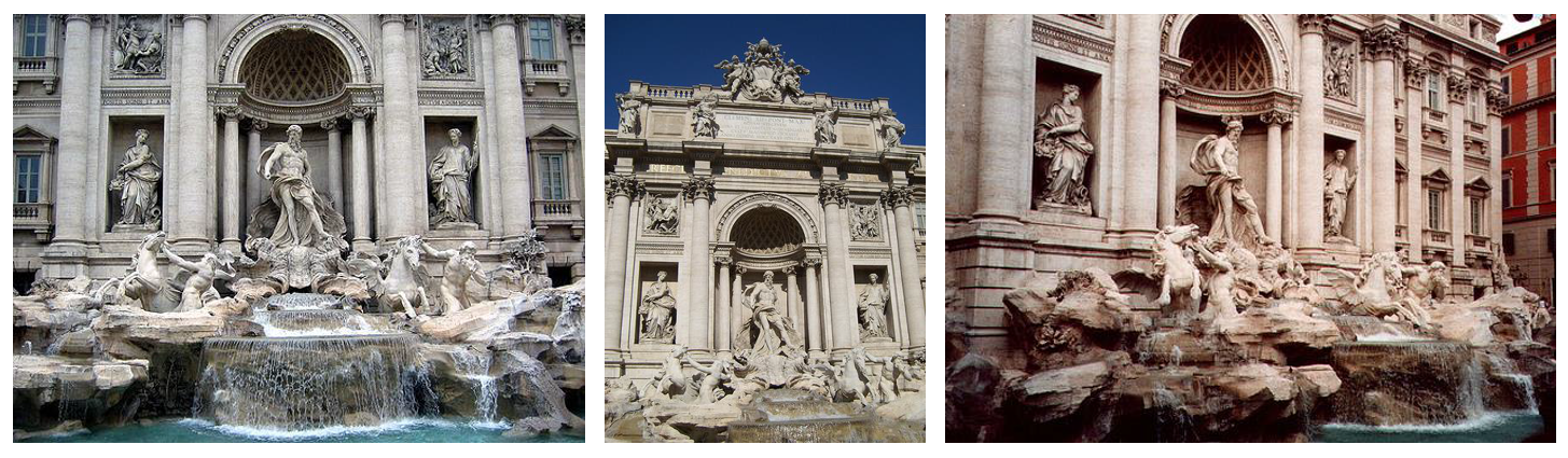
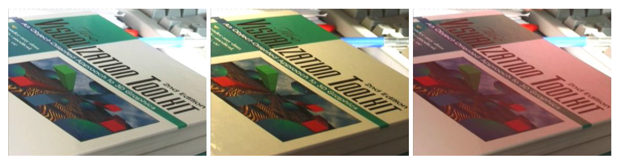
场景1：光照的大幅变化

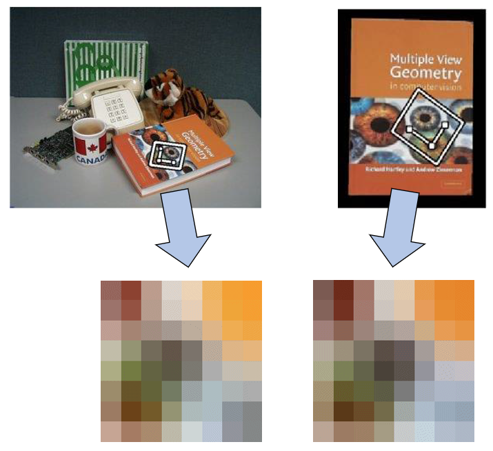
场景2：视场角、距离的大幅变化

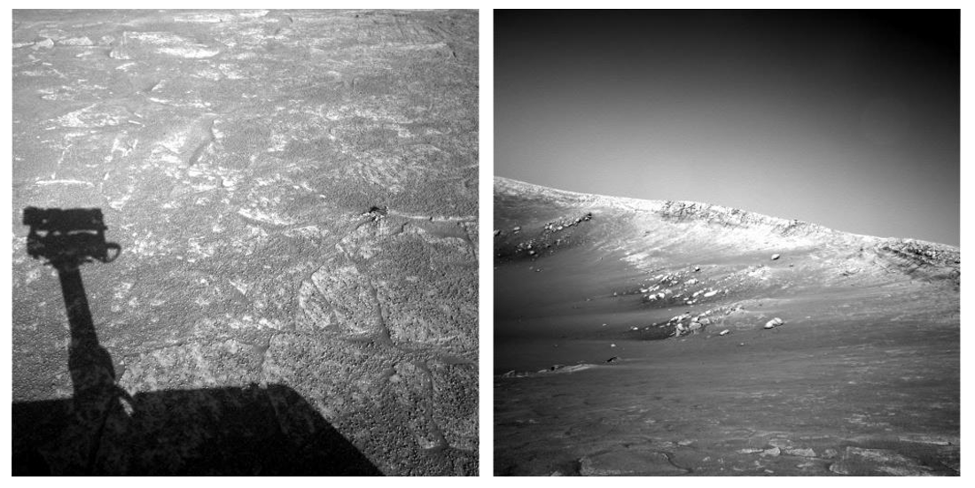
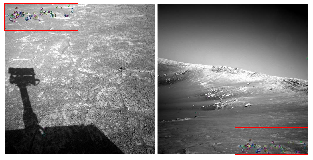
对于场景1，光照的变化，大家肯定还能分辨出场景中的相同部分，但对场景2，绝大多数人甚至没法进行直观视觉上的区域匹配。这个问题就是有这么离谱，人都分辨不出来，还能交给计算机去完成吗，答案是可以，结果如下。

我们可以总结一下，我们需要什么样的特征，或者说一个好的特征应该满足哪些条件。

1.几何不变：不因几何形变而改变

2.光照不变：不因光照的改变而改变

3.可重复与准确度：重复提取特征，结果不会发生改变，同时准确度高

4.数量足够：需要较多数量的点来覆盖一块区域

5.特征性：每个特征都要独一无二，有明显特点利于区分

由此，我们已经明确了何为图像特征，以及图像特征最好能够具有的性质。

3 Harris角点检测

目的：

可重复检测
精确定位
包含图像的高频信息

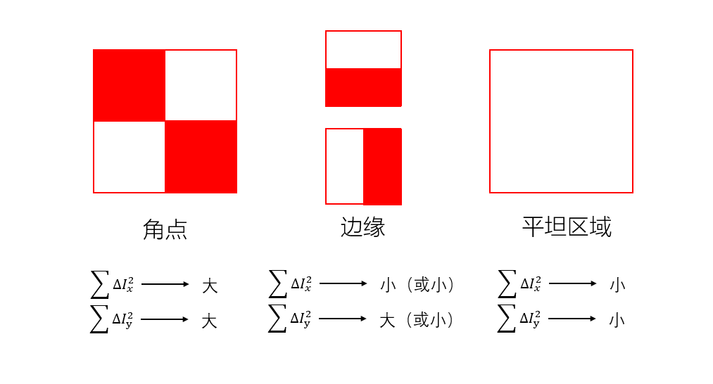
本质：寻找图像的二维信号变化，在角点区域附近，图像的梯度有两个或更多的变化方向。

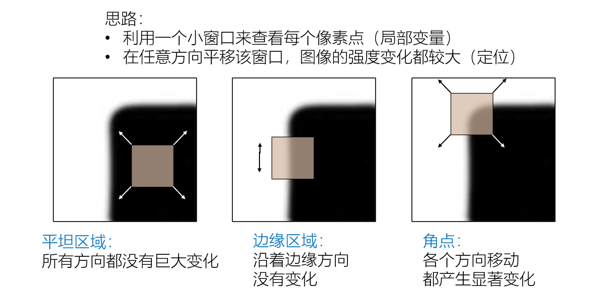
而角点有如下的数理规律：

对于平坦区域，在水平和竖直方向上的梯度小；对于边缘区域，在水平和竖直两个方向上有一者梯度大，一者梯度小；对于角点，则在两个方向上都有较大的梯度。下图较形象地描述了三者的区别。

3.1 Harris角点检测的数学表达

将图像平移 $(u,v)$ 产生灰度变化 $E(u,v)$ ，如下：

E(u,v)=\sum_{x,y}w(x,y) \left[ I(x+u,y+v)-I(x,y)\right]^2

由泰勒展开，得

I(x+u,y+v)=I(x,y)+I_x(x,y)u+I_y(x,y)v+O(u^2,v^2)

则

E(u,v)=\sum_{x,y}w(x,y) \left[ I_x(x,y)u+I_y(x,y)v+O(u^2,v^2)\right]^2

其中项 $O(u^2.v^2)$ 可以被近似认为是0，因此

E(u,v)\approx \sum_{x,y}w(x,y) \left[ I_x(x,y)u+I_y(x,y)v\right]^2

二次项展开

E(u,v)\approx \sum_{x,y}w(x,y) \left[ I_x^2u^2+I^2_yv^2+2I_xI_yuv\right]

该式用矩阵来表示为：

[I_xu+I_yv]^2\approx[u,v] \left[ \begin{matrix}
I_x^2 & I_xI_y \\ I_xI_y & I_y^2 \end{matrix} \right] \left[\begin{matrix}u\\v \end{matrix}\right]

此表达式即为

E(u,v)\approx [u,v] M \left[\begin{matrix}u\\v \end{matrix}\right]

在编程的时候，我们将M当作一个2x2的矩阵，可以由图像的梯度计算而来

M=\sum\left[ \begin{matrix}
I_x \\I_y \end{matrix} \right] \left[ I_x,I_y\right]=\left[ \begin{matrix}
\lambda_1 & 0 \\ 0 & \lambda_2 \end{matrix} \right]

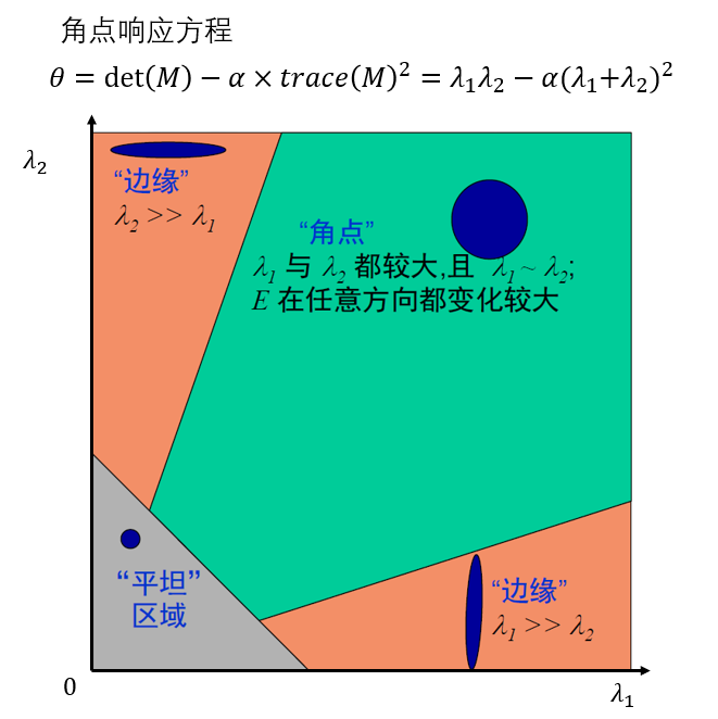
观察一下上式，它表明：

主要梯度变化方向沿着x方向或y方向
如果任意一个 $\lambda$ 接近于0，那么这就不是一个角，因此只有两个 $\lambda$ 都较大才是角点。

3.2 Harris角点检测示例

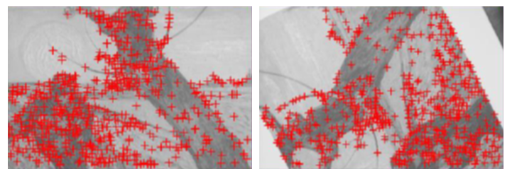
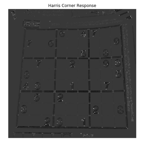
对于一幅输入图像，其经过非极大值抑制的Harris角点响应图如下。（代码部分详见代码实战部分与实施例）

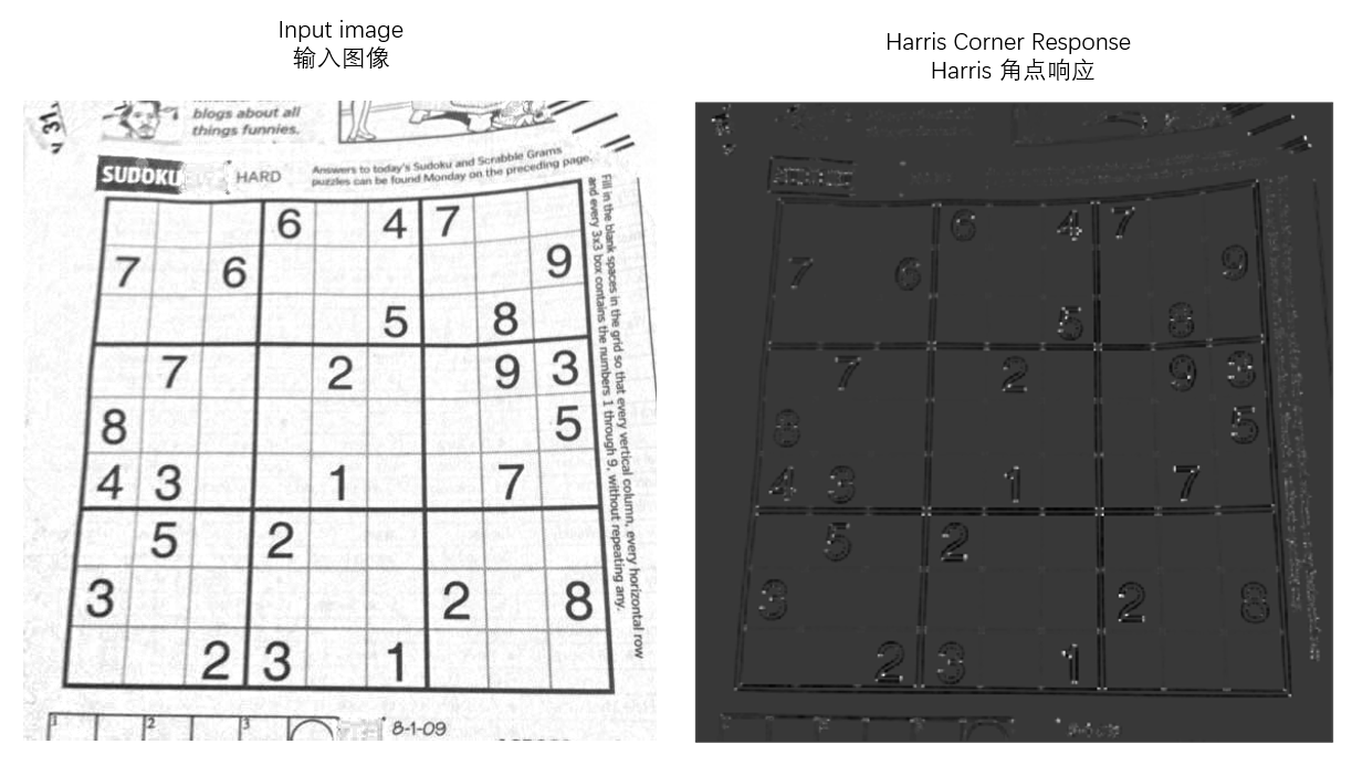
其中，亮点与红点区域即为Harris角点计算所得的角点区域。

Harris角点检测可以保证图像特征的平移不变性、旋转不变性、强度（光照）不变性，但缺陷在于无法保证尺度不变（缩放不变），因此对于不同的窗口大小，能够检测出的角点有所不同。这就导致了特征因拍摄距离的变化而发生变化，无法做到特征的稳定性。

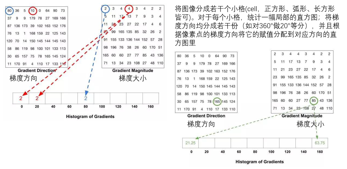
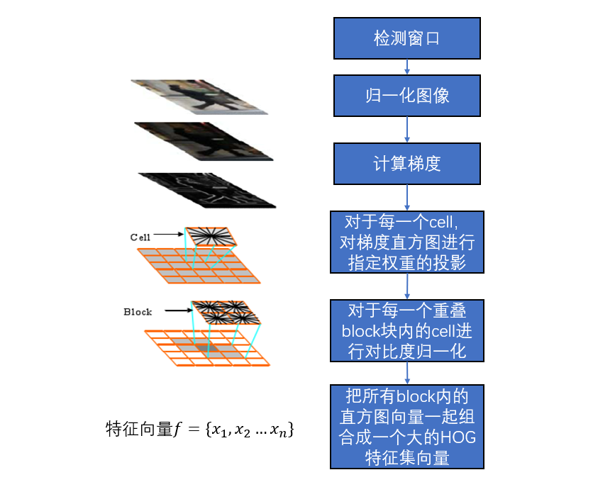
4 方向梯度直方图(Histogram of Oriented Gradients, HOG)

目标：

寻找一组稳定的特征用以分辨物体（主要是人）
主要用于图像的整体描述（图片中的滑动窗口）

难点：

形状与外貌变化太广
不同的照明条件下，背景过于庞杂
实时处理速度有所限制

HOG背后的原理涉及数学的部分较少，我们可以用过程形象地说其作用原理。

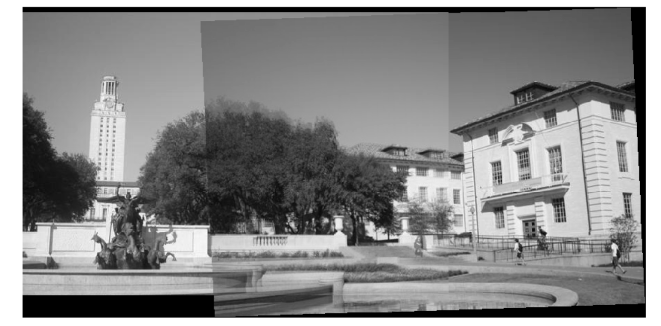
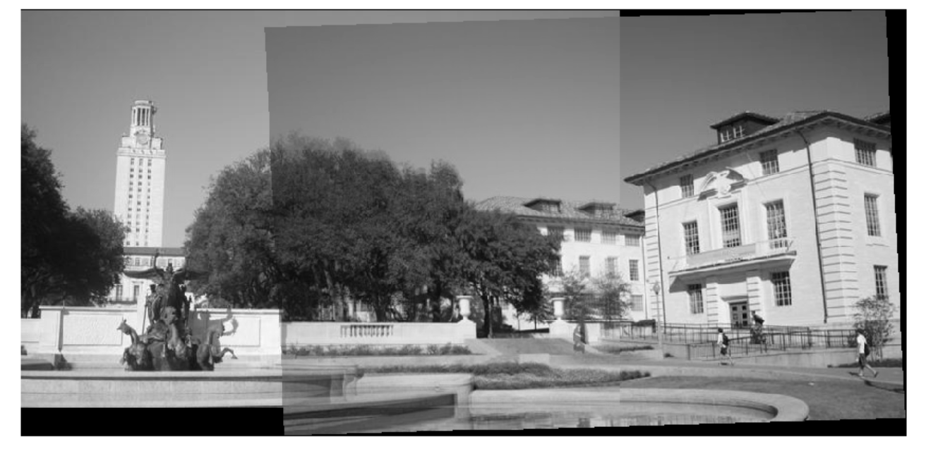
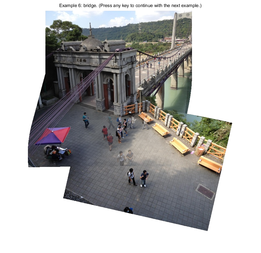
5 图像特征的应用：相机中全景图像的计算成像

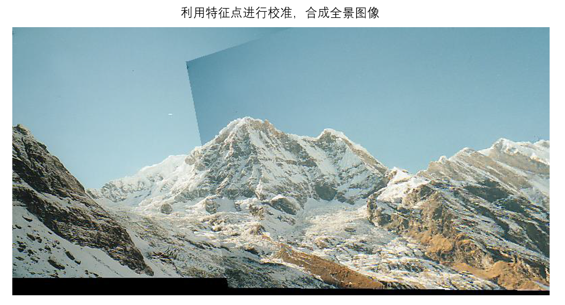
此处的合成图像过渡不平滑，是因为成像过程中镜头的进光量等因素的变化所导致的，解决该问题有许多方法，如图像金字塔融合、加权融合等，这不是本文重点。

6 代码实战部分

# Python 3.6
# panorama.py


import numpy as np
from skimage import filters
from skimage.feature import corner_peaks
from skimage.util.shape import view_as_blocks
from scipy.spatial.distance import cdist
from scipy.ndimage.filters import convolve

from utils import pad, unpad, get_output_space, warp_image


def harris_corners(img, window_size=3, k=0.04):
    """
    计算图像的Harris角点值，其计算公式如下：
    R=Det(M)-k(Trace(M)^2).

    提示:
        你可以利用卷积函数 scipy.ndimage.filters.convolve。

    参数:
        img: 形状为 (H, W)的灰度图
        window_size: kernel的尺寸
        k: 敏感度调节因子

    返回值:
        response: 图像的角点响应值 (H, W)
    """
    #img = img[:,:,0]   #如果29行报错，请把28行的img = [:,:,0]的注释取消
    H, W = img.shape
    window = np.ones((window_size, window_size))

    response = np.zeros((H, W))

    dx = filters.sobel_v(img)
    dy = filters.sobel_h(img)
    
    
    ### YOUR CODE HERE
    #M = np.ones((H, W,2, 2))
    #padded_dx = np.pad(dx, int((window_size-1)/2), mode='edge')
    #padded_dy = np.pad(dy, int((window_size-1)/2), mode='edge')
    #for i in range(H):
        #for j in range(W):
            #M[i, j, :, :] = np.array([[sum(sum(b) for b in (padded_dx[i:i+2, j:j+2]*padded_dx[i:i+2, j:j+2])),sum(sum(b) for b in (padded_dx[i:i+2, j:j+2]*padded_dy[i:i+2, j:j+2]))],[sum(sum(b) for b in (padded_dx[i:i+2, j:j+2]*padded_dy[i:i+2, j:j+2])),sum(sum(b) for b in (padded_dy[i:i+2, j:j+2]*padded_dy[i:i+2, j:j+2]))]])
    #for a in range(H):
        #for b in range(W):
            #response[a][b]=np.linalg.det(M[a][b])-k*(np.trace(M[a][b])**2)

    dxx = dx * dx
    dyy = dy * dy
    dxy = dx * dy
    mxx = convolve(dxx, window)
    mxy = convolve(dxy, window)
    myy = convolve(dyy, window)    
    for i in range(H):
        for j in range(W):
            M = np.array([[mxx[i, j], mxy[i, j]], [mxy[i, j], myy[i, j]]])
            response[i, j] = np.linalg.det(M) - k * np.trace(M) ** 2
    ### END YOUR CODE
    return response


def simple_descriptor(patch):
    """
    将像素值分布进行标准正态化来描述这个小patch (标准正态分布的均值为0，标准差为1)，
    然后将它展开成一维的数组.

    正态化的操作会使描述子对于光照变化更加robust.

    提示:
        如果分母为0，那就用1来代替.

    Args:
        patch: 尺寸为 (H, W)的灰度图像

    Returns:
        feature: 尺寸为 (H * W)的一维数组
    """
    feature = []
    ### YOUR CODE HERE
    patch = patch.reshape(-1)
    mean = np.mean(patch)     
    delta = np.std(patch)    
    if delta > 0.0:
        patch = (patch - mean) / delta
    else:
        patch = patch - mean
    feature = list(patch)
    ### END YOUR CODE
    return feature


def describe_keypoints(image, keypoints, desc_func, patch_size=16):
    """
    Args:
        image: 尺寸为 (H, W)的灰度图
        keypoints: 二维数组，每一行都包含一个关键点 (y, x)。
        desc_func: 特征描述函数，输入一张图，输出为它所对应的描述算子
        patch_size: 每个特征点所对应的局部图像的尺寸。为了简化，这里将长宽设定成相同。

    Returns:
        desc: 描述各个特征点的特征向量
    """

    image.astype(np.float32)
    desc = []

    for i, kp in enumerate(keypoints):
        y, x = kp
        patch = image[y-(patch_size//2):y+((patch_size+1)//2),
                      x-(patch_size//2):x+((patch_size+1)//2)]
        desc.append(desc_func(patch))
    return np.array(desc)


def match_descriptors(desc1, desc2, threshold=0.5):
    """
    通过计算两点之间的欧氏距离来完成特征点的匹配. 现在，我们有两组特征向量。
    从第一组中任选一个特征向量v1，计算它与第二组每个特征向量之间的距离，我们就得到了v1与其他特征向量之间的距离。
    如果离v1最近的特征向量分别是v21,v22,那么，如果v1和v21的距离远小于v1和v22的距离，那么，我们认为v1和v21就是一组。
    也就是说d(v1,v21)/d(v1,v22)需要小于某个阈值(threshold)。
    据此，我们可以找出所有的匹配点。

    提示:
        Numpy 里的函数 np.sort, np.argmin, np.asarray 可能会对计算有帮助。

    Args:
        desc1: 形状为 (M, P)的数组，它的每一行都是一个描述子(尺寸为P)，共有M个特征向量（M个特征点）。
        desc2: 形状为 (N, P)的数组，它的每一行都是一个描述子(尺寸为P)，共有N个特征向量（N个特征点）。

    Returns:
        matches: 尺寸为 (Q, 2) 的数组。它的每一行都是一组匹配的特征点序号(indices of one pair
        of matching descriptors)。
    """
    matches = []

    N = desc1.shape[0]
    dists = cdist(desc1, desc2)     # 每个向量的欧式距离 N * N
    ### YOUR CODE HERE
    #M = desc2.shape[1]

    idx = np.argsort(dists, axis=1)  
    for i in range(N):
        closed_dist = dists[i, idx[i, 0]]
        second_dist = dists[i, idx[i, 1]]
        if(closed_dist < threshold * second_dist):  
            matches.append([i, idx[i, 0]])

    matches = np.array(matches)
    ### END YOUR CODE
    return matches


def fit_affine_matrix(p1, p2):
    """ 拟合 affine变换矩阵，使得 p2 * H = p1

    提示:
        你可以使用 np.linalg.lstsq 函数来求解这个问题.

    Args:
        p1: 尺寸为 (M, P) 的矩阵，每一行代表一个特征点的坐标
        p2: 尺寸为 (M, P) 的矩阵，每一行代表一个特征点的坐标

    Return:
        H: 尺寸为 (P, P) 的矩阵，他将p2转换到p1。
    """

    assert (p1.shape[0] == p2.shape[0])

    p1 = pad(p1)
    p2 = pad(p2)
    
    ### YOUR CODE HERE

    H = np.linalg.lstsq(p2, p1)[0]
    ### END YOUR CODE
    # 有时候由于噪声影响，会使得最后一列不是精确的[0, 0, 1]，此时我们可以手动将它置为[0, 0, 1]
    H[:,2] = np.array([0, 0, 1])
    return H


def ransac(keypoints1, keypoints2, matches, n_iters=200, threshold=20):
    """
    利用 RANSAC 来找到一组robust的affine变换

        1. 随机选取若干组match点(对于affine变换，至少需要选取三组match，想想这是为什么？)
        2. 计算affine的变换矩阵
        3. 计算有效数据点(inliers)的数目
        4. 记录有效点数目最大的那组参数
        5. 根据所有的有效点，重新计算一遍变换矩阵

    Args:
        keypoints1: M1 x 2 矩阵，每一行都是一个像素点
        keypoints2: M2 x 2 矩阵，每一行都是一个像素点
        matches: N x 2 的矩阵，每一行都代表一组match
            [keypoint1的序号, keypoint 2的序号]
        n_iters: RANSAC算法要进行循环的次数。为了简化计算，这里将循环次数固定到了200。
            (想想我们上课时候讲过如何确定循环次数？在不知道数据好坏的情况下，如何动态地改变循环次数？)
        threshold: 有效数据点个数的阈值
    
    提示：np.random.choice函数可能会有帮助

    Returns:
        H: 对于affine变换的一个robust的估计，它将 keypoints2 变换到了 keypoints 1
    """
    # 保存match数组，避免对它直接改写
    orig_matches = matches.copy()
    matches = matches.copy()

    N = matches.shape[0]
    print(N)
    n_samples = int(N * 0.2) #这里将n_samples的值与N联系起来。对于affine变换，你也可以将它固定到3.

    matched1 = pad(keypoints1[matches[:,0]])
    matched2 = pad(keypoints2[matches[:,1]])

    max_inliers = np.zeros(N)
    n_inliers = 0
    
     # 开始对RANSAC 算法进行循环
    ### YOUR CODE HERE
    for i in range(n_iters):

        temp_max = np.zeros(N, dtype=np.int32)     
        temp_n = 0

        idx = np.random.choice(N, n_samples, replace=False)    
        p1 = matched1[idx, :]
        p2 = matched2[idx, :]
        H = np.linalg.lstsq(p2, p1)[0]           
        H[:, 2] = np.array([0, 0, 1])

        temp_max = np.linalg.norm(matched2.dot(H) - matched1, axis=1) ** 2 < threshold    
        temp_n = np.sum(temp_max)

        if temp_n > n_inliers:      
            max_inliers = temp_max.copy()
            n_inliers = temp_n

    H = np.linalg.lstsq(matched2[max_inliers], matched1[max_inliers])[0]
    H[:, 2] = np.array([0, 0, 1])
    ### END YOUR CODE
    print(H)
    return H, matches[max_inliers]


def hog_descriptor(patch, pixels_per_cell=(8,8)):
    """
    按照如下步骤生成HOG描述符:

    1. 计算x- 以及 y-方向的梯度图像 (已经算好了)
    2. 对于每个cell，计算梯度直方图
    3. 对于每个block，将它们平铺成一维的向量。
        在此, 我们将整个patch都视作一个block
    4. 将平铺后的block进行标准正态化
        正态化会使得描述子对于光照变化更加robust

    参数:
        patch: 尺寸为 (H, W) 的灰度图
        pixels_per_cell: 每个cell的尺寸 (M, N)
        
    提示：
        你可能会用到view_as_blocks函数

    Returns:
        block: 一维向量，表征该patch的特征描述向量，尺寸为： ((H*W*n_bins)/(M*N))
    """
    assert (patch.shape[0] % pixels_per_cell[0] == 0),\
                'Heights of patch and cell do not match'
    assert (patch.shape[1] % pixels_per_cell[1] == 0),\
                'Widths of patch and cell do not match'

    n_bins = 9
    degrees_per_bin = 180 // n_bins

    Gx = filters.sobel_v(patch)
    Gy = filters.sobel_h(patch)

    # 无符号梯度
    G = np.sqrt(Gx**2 + Gy**2)
    theta = (np.arctan2(Gy, Gx) * 180 / np.pi) % 180

    # 将尺寸为(M, N)的cell视作一个像素点
    #   G_cells.shape = theta_cells.shape = (H//M, W//N)
    #   G_cells[0, 0].shape = theta_cells[0, 0].shape = (M, N)

    G_cells = view_as_blocks(G, block_shape=pixels_per_cell)
    theta_cells = view_as_blocks(theta, block_shape=pixels_per_cell)
    rows = G_cells.shape[0]
    cols = G_cells.shape[1]

    # 对于每个cell, 计算梯度直方图。它的尺寸是n_bins
    cells = np.zeros((rows, cols, n_bins))

    # 对于每个cell，计算梯度直方图
    ### YOUR CODE HERE

    # Compute histogram per cell
    for i in range(rows):
        for j in range(cols):
            for m in range(pixels_per_cell[0]):
                for n in range(pixels_per_cell[1]):
                    idx = int(theta_cells[i, j, m, n] // degrees_per_bin)  
                    if idx == 9:   
                        idx = 8
                    cells[i, j, idx] += G_cells[i, j, m, n]            

    cells = (cells - np.mean(cells)) / np.std(cells)      
    block = cells.reshape(-1)
    ### YOUR CODE HERE
    return block


def linear_blend(img1_warped, img2_warped):
    """
    按照下列步骤，将图片 img1_warped 和图片 img2_warped 进行线性混合:

    1. 确定 left 和 right 空白位置 (已经帮你完成)
    2. 为img1_warped 和 img2_warped分别确定一个权重矩阵
        你可能会用到np.linspace 和 np.tile 函数
    3. 将权重矩阵分别应用到它们对应的图片里
    4. 将图像合并到一起

    Args:
        img1_warped: 输出图像里img1的部分
        img2_warped: 输出图像里img2的部分

    Returns:
        merged: 融合到一起的图像
    """
    out_H, out_W = img1_warped.shape # 输出图像的尺寸
    img1_mask = (img1_warped != 0)  # Mask == 1 inside the image
    img2_mask = (img2_warped != 0)  # Mask == 1 inside the image

    # 找出img1在输出图像里面最右边的column
    # 这是我们img1权重矩阵的终点（也就是权重值为0所对应的位置）
    right_margin = out_W - np.argmax(np.fliplr(img1_mask)[out_H//2, :].reshape(1, out_W), 1)[0]

    # 找出img2在输出图像里面最左边的column
    # 这是我们img2权重矩阵的起点（也就是权重值为1所对应的位置）
    left_margin = np.argmax(img2_mask[out_H//2, :].reshape(1, out_W), 1)[0]

    ### YOUR CODE HERE
    left_matrix = np.array(img1_mask,  dtype=np.float64)     
    right_matrix = np.array(img2_mask, dtype=np.float64)
    left_matrix[:, left_margin: right_margin] = np.tile(np.linspace(1, 0, right_margin - left_margin), (out_H, 1))
    right_matrix[:, left_margin: right_margin] = np.tile(np.linspace(0, 1, right_margin - left_margin), (out_H, 1))
    img1 = left_matrix * img1_warped
    img2 = right_matrix * img2_warped
    merged = img1 + img2
    ### END YOUR CODE
    return merged


def stitch_multiple_images(imgs, desc_func=simple_descriptor, patch_size=5):
    """
    将一系列图片拼接到一起.

    参数:
        imgs: 长度为m的List，每个元素都是图片，并且图片是有序排列的。
        desc_func: 特征描述函数，输入一张图，输出为它所对应的描述算子
        patch_size: 每个特征点所对应的局部图像的尺寸。为了简化，这里将长宽设定成相同。

    Returns:
        panorama: 最终生成的全景图
    """
    # 对于每张照片，检测其特征点
    keypoints = []  # keypoints[i] 对应于 imgs[i]
    for img in imgs:
        kypnts = corner_peaks(harris_corners(img, window_size=3),
                              threshold_rel=0.05,
                              exclude_border=8)
        keypoints.append(kypnts)
    # 描述特征点
    descriptors = []  # descriptors[i] 对应于 keypoints[i]
    for i, kypnts in enumerate(keypoints):
        desc = describe_keypoints(imgs[i], kypnts,
                                  desc_func=desc_func,
                                  patch_size=patch_size)
        descriptors.append(desc)
    # 将相邻图片的特征点匹配到一起
    matches = []  # matches[i] 记录了 descriptors[i] 与 descriptors[i+1]的match点
    H = []
    robust_matches = []
    for i in range(len(imgs)-1):
        mtchs = match_descriptors(descriptors[i], descriptors[i+1], 0.7)
        matches.append(mtchs)
        h, robust_m = ransac(keypoints[i], keypoints[i+1], matches[i])
        H.append(h)
        robust_matches.append(robust_m)
    #利用match的像素点完成图像的拼接
    ### YOUR CODE HERE
        
    output_shape, offset = get_output_space(imgs[1], [imgs[0], imgs[2], imgs[3]],
                                            [np.linalg.inv(H[0]), H[1], np.dot(H[1],H[2])])

    img1_warped = warp_image(imgs[0], np.linalg.inv(H[0]), output_shape, offset)
    img1_mask = (img1_warped != -1) 
    img1_warped[~img1_mask] = 0  

    img2_warped = warp_image(imgs[1], np.eye(3), output_shape, offset)
    img2_mask = (img2_warped != -1)  
    img2_warped[~img2_mask] = 0  

    img3_warped = warp_image(imgs[2], H[1], output_shape, offset)
    img3_mask = (img3_warped != -1)  
    img3_warped[~img3_mask] = 0 

    img4_warped = warp_image(imgs[3], np.dot(H[1], H[2]), output_shape, offset)
    img4_mask = (img4_warped != -1)  
    img4_warped[~img4_mask] = 0  

    panorama = linear_blend(img1_warped, img2_warped)
    panorama = linear_blend(panorama, img3_warped)
    panorama = linear_blend(panorama, img4_warped)
    ### END YOUR CODE
    return panorama

# Python 3.6
# utils.py

import numpy as np
from scipy.ndimage import affine_transform

# 完成欧式坐标与齐次坐标之间的转换
pad = lambda x: np.hstack([x, np.ones((x.shape[0], 1))])
unpad = lambda x: x[:,:-1]

def plot_matches(ax, image1, image2, keypoints1, keypoints2, matches,
                 keypoints_color='k', matches_color=None, only_matches=False):
    """将匹配的特征点给绘制出来.
    参数
    ----------
    ax : matplotlib.axes.Axes
        坐标轴，用于绘制图像以及匹配点对.
    image1 : (N, M [, 3]) array
        灰度图或者彩色图像.
    image2 : (N, M [, 3]) array
        灰度图或者彩色图像.
    keypoints1 : (K1, 2) array
        图1的关键点 ``(row, col)``.
    keypoints2 : (K2, 2) array
        图2的关键点 ``(row, col)``.
    matches : (Q, 2) array
        match点对的序号。
        每一行第一个值是keypoints1的序号，第二个值是keypoints2的序号
    keypoints_color : matplotlib color, optional
        指定绘制的颜色，可选.
    matches_color : matplotlib color, optional
        两点连线的颜色.
    only_matches : bool, optional
        是否绘制keypoint点的坐标.
    """

    image1.astype(np.float32)
    image2.astype(np.float32)

    new_shape1 = list(image1.shape)
    new_shape2 = list(image2.shape)

    if image1.shape[0] < image2.shape[0]:
        new_shape1[0] = image2.shape[0]
    elif image1.shape[0] > image2.shape[0]:
        new_shape2[0] = image1.shape[0]

    if image1.shape[1] < image2.shape[1]:
        new_shape1[1] = image2.shape[1]
    elif image1.shape[1] > image2.shape[1]:
        new_shape2[1] = image1.shape[1]

    if new_shape1 != image1.shape:
        new_image1 = np.zeros(new_shape1, dtype=image1.dtype)
        new_image1[:image1.shape[0], :image1.shape[1]] = image1
        image1 = new_image1

    if new_shape2 != image2.shape:
        new_image2 = np.zeros(new_shape2, dtype=image2.dtype)
        new_image2[:image2.shape[0], :image2.shape[1]] = image2
        image2 = new_image2

    image = np.concatenate([image1, image2], axis=1)

    offset = image1.shape

    if not only_matches:
        ax.scatter(keypoints1[:, 1], keypoints1[:, 0],
                   facecolors='none', edgecolors=keypoints_color)
        ax.scatter(keypoints2[:, 1] + offset[1], keypoints2[:, 0],
                   facecolors='none', edgecolors=keypoints_color)

    ax.imshow(image, interpolation='nearest', cmap='gray')
    ax.axis((0, 2 * offset[1], offset[0], 0))

    for i in range(matches.shape[0]):
        idx1 = matches[i, 0]
        idx2 = matches[i, 1]

        if matches_color is None:
            color = np.random.rand(3)
        else:
            color = matches_color

        ax.plot((keypoints1[idx1, 1], keypoints2[idx2, 1] + offset[1]),
                (keypoints1[idx1, 0], keypoints2[idx2, 0]),
'-', color=color)


def get_output_space(img_ref, imgs, transforms):
    """
    Args:
        img_ref: 参考图(reference image)
        imgs: 需要被变换的图片(images to be transformed)
        transforms: affine变换矩阵所组成的一个List. transforms[i] 将图片 imgs[i]中的点 map 到 img_ref
    Returns:
        输出image的尺寸
    """

    assert (len(imgs) == len(transforms))

    r, c = img_ref.shape
    corners = np.array([[0, 0], [r, 0], [0, c], [r, c]])
    all_corners = [corners]

    for i in range(len(imgs)):
        r, c = imgs[i].shape
        H = transforms[i]
        corners = np.array([[0, 0], [r, 0], [0, c], [r, c]])
        warped_corners = corners@H[:2,:2] + H[2,:2]
        all_corners.append(warped_corners)

    # 找出Corner的边界
    all_corners = np.vstack(all_corners)

    # 整幅输出图的形状是两个最远的conrner相减
    corner_min = np.min(all_corners, axis=0)
    corner_max = np.max(all_corners, axis=0)
    output_shape = (corner_max - corner_min)

    # 确保输出是整数
    output_shape = np.ceil(output_shape).astype(int)
    offset = corner_min

    return output_shape, offset

def warp_image(img, H, output_shape, offset):

    # 需要注意 affine_transfomr 这个函数:
    # 给定一个输出图像的像素点 o,
    # 它的像素值是由下式所决定的：
    # np.dot(matrix,o) + offset.
    # 因此, 我们需要将转换矩阵求一个逆.
    # 这样反向求的好处是，插值更加方便。
    Hinv = np.linalg.inv(H)
    m = Hinv.T[:2,:2]
    b = Hinv.T[:2,2]
    img_warped = affine_transform(img.astype(np.float32),
                                  m, b+offset,
                                  output_shape,
                                  cval=-1)

    return img_warped

7 实施例

7.1 Harris角点部分

我们首先从Harris角点检测开始

# 初始化配置
import numpy as np
from skimage import filters
from skimage.feature import corner_peaks
from skimage.io import imread
import matplotlib.pyplot as plt
from time import time
from panorama import harris_corners


%matplotlib inline
plt.rcParams['figure.figsize'] = (15.0, 12.0) # 设置默认尺寸
plt.rcParams['image.interpolation'] = 'nearest'
plt.rcParams['image.cmap'] = 'gray'

# 自动重装外部模块
%load_ext autoreload
%autoreload 2

img = imread('sudoku.png', as_gray=True)

# 计算Harris角点响应值
response = harris_corners(img)

# 显示角点响应值
plt.imshow(response)
plt.axis('off')
plt.title('Harris Corner Response')

# 对Harris响应图片进行非极大值抑制
# 然后输出响应点的坐标
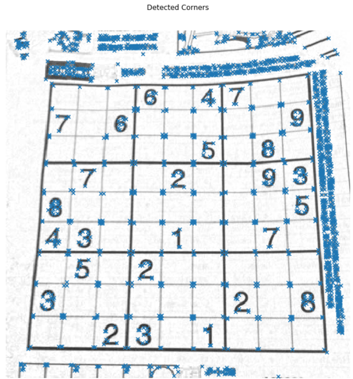
corners = corner_peaks(response, threshold_rel=0.01)

# 显示角点
plt.imshow(img)
plt.scatter(corners[:,1], corners[:,0], marker='x')
plt.axis('off')
plt.title('Detected Corners')
plt.show()

from panorama import harris_corners

img1 = imread('uttower1.jpg', as_grey=True)
img2 = imread('uttower2.jpg', as_grey=True)

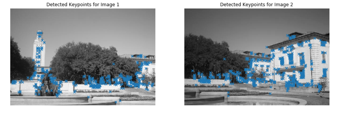
# 利用Harris角点检测算法检测两张图片中的关键点
keypoints1 = corner_peaks(harris_corners(img1, window_size=3),
                          threshold_rel=0.05,
                          exclude_border=8)
keypoints2 = corner_peaks(harris_corners(img2, window_size=3),
                          threshold_rel=0.05,
                          exclude_border=8)

# 显示检测到的关键点
plt.subplot(1,2,1)
plt.imshow(img1)
plt.scatter(keypoints1[:,1], keypoints1[:,0], marker='x')
plt.axis('off')
plt.title('Detected Keypoints for Image 1')

plt.subplot(1,2,2)
plt.imshow(img2)
plt.scatter(keypoints2[:,1], keypoints2[:,0], marker='x')
plt.axis('off')
plt.title('Detected Keypoints for Image 2')
plt.show()

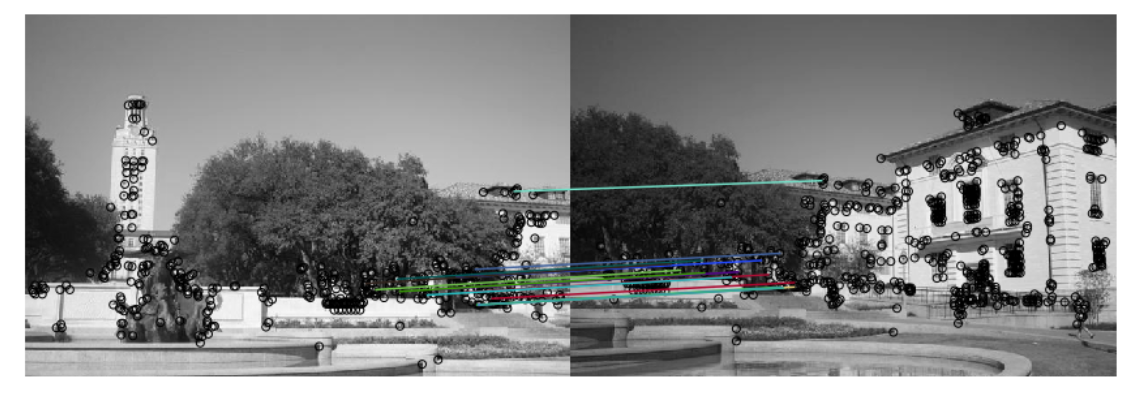
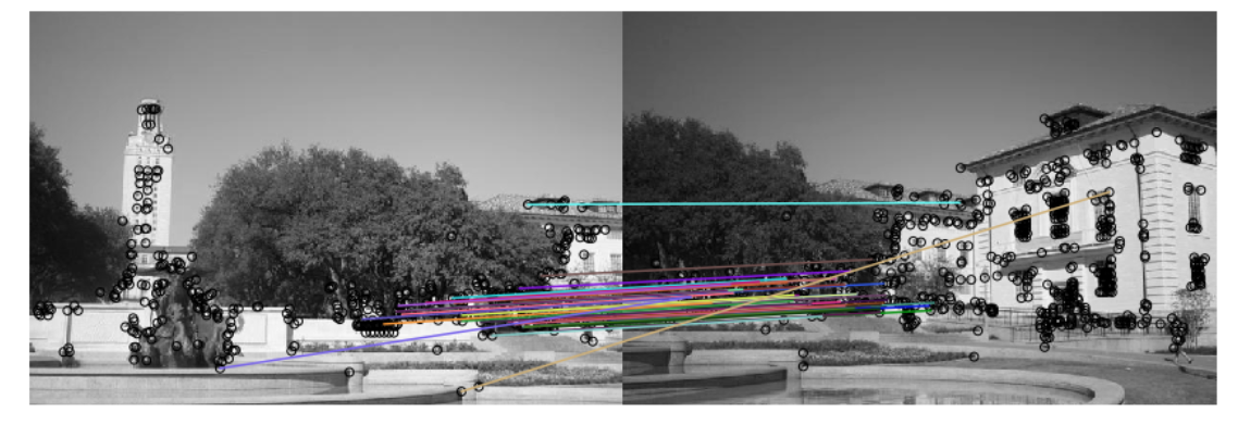
由此，得到了角点特征，我们需要进行匹配描述。找到两组描述子集合中相匹配的向量。首先，从两张图片中各取一个描述子（也就是关键点生成的向量），计算它们的欧氏距离。利用欧氏距离来判定它们是不是对应的一组描述子:如果这一对描述子的距离显著小于其他的距离，那么我们认为它们是一组对应的特征点。该函数的输出会是一组数列（array），数列的每一行都是一组对应的描述子索引号(index)。

from panorama import simple_descriptor, match_descriptors, describe_keypoints
from utils import plot_matches

patch_size = 5
    
# 利用关键点生成描述向量(描述子)
desc1 = describe_keypoints(img1, keypoints1,
                           desc_func=simple_descriptor,
                           patch_size=patch_size)
desc2 = describe_keypoints(img2, keypoints2,
                           desc_func=simple_descriptor,
                           patch_size=patch_size)

# 将描述子进行匹配
matches = match_descriptors(desc1, desc2, 0.7)

# 画出匹配的点
fig, ax = plt.subplots(1, 1, figsize=(15, 12))
ax.axis('off')
plot_matches(ax, img1, img2, keypoints1, keypoints2, matches)
plt.show()

现在，我们已经有一组描述子的对应列表。我们将利用这组对应列表计算从图片二映射到图片一的变换矩阵。换句话说，如果图片1中的点 $p1=[y1,x1]$ 与图片2中的点 $p2=[y2,x2]$ 相匹配, 我们需要找出一个仿射变换矩阵来进行坐标变换，使得

其中， $\widetilde p_1$ 和 $\widetilde p_2$ 都是齐次坐标。

需要注意的是，矩阵 $H$ 很有可能不能使得每一组对应点都完全匹配，但是我们可以利用最小二乘法来进行估计最优的矩阵H。假设给定了 $N$ 组匹配的特征点,让 $X_1$ 和 $X_2$ 为两个 $N×3$ 的矩阵，矩阵的每一行都是对应特征点的齐次坐标（也就是原坐标后面补1）。那么，我们知道矩阵 $H$ 应该满足条件：

from panorama import fit_affine_matrix

# 检查变换矩阵求解是否正确

# 测试值
a = np.array([[0.5, 0.1], [0.4, 0.2], [0.8, 0.2]])
b = np.array([[0.3, -0.2], [-0.4, -0.9], [0.1, 0.1]])

H = fit_affine_matrix(b, a)

# 期望的输出值
sol = np.array(
    [[1.25, 2.5, 0.0],
     [-5.75, -4.5, 0.0],
     [0.25, -1.0, 1.0]]
)

error = np.sum((H - sol) ** 2)

if error < 1e-20:
    print('Implementation correct!')
else:
    print('There is something wrong.')

from utils import get_output_space, warp_image

# 获取特征点
p1 = keypoints1[matches[:,0]]
p2 = keypoints2[matches[:,1]]

# 求解变换矩阵
H = fit_affine_matrix(p1, p2)

output_shape, offset = get_output_space(img1, [img2], [H])
print("Output shape:", output_shape)
print("Offset:", offset)


# 进行坐标变换
img1_warped = warp_image(img1, np.eye(3), output_shape, offset)# 图片1没变，因此用单位阵作为变换矩阵
img1_mask = (img1_warped != -1) # Mask不等于-1表示该位置为原图片插值后的点
img1_warped[~img1_mask] = 0     # Mask取反表示在该位置没有值（该位置为背景），置0使得该位置变黑

img2_warped = warp_image(img2, H, output_shape, offset)
img2_mask = (img2_warped != -1) # Mask不等于-1表示该位置为原图片插值后的点
img2_warped[~img2_mask] = 0     # Mask取反表示在该位置没有值（该位置为背景），置0使得该位置变黑

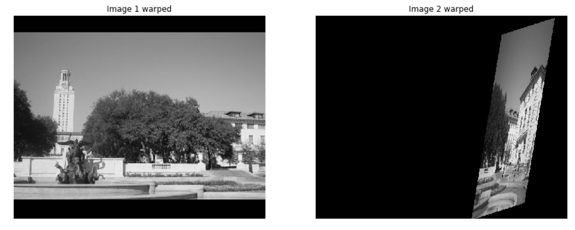
# 画出坐标变换后的图像
plt.subplot(1,2,1)
plt.imshow(img1_warped)
plt.title('Image 1 warped')
plt.axis('off')

plt.subplot(1,2,2)
plt.imshow(img2_warped)
plt.title('Image 2 warped')
plt.axis('off')

plt.show()

运行输出结果：Output shape: [496 615]

Offset: [-39.37184617 0. ]

现在，其实我们已经发现结果貌似有点不太正常，不过没关系，我们先往下做，最后再进行结果分析。我们可以将两幅经过坐标变换的图片拼接成一张。

merged = img1_warped + img2_warped

# 确定哪些值被加了两次
overlap = (img1_mask * 1.0 +  # bool 型转成 float 
           img2_mask)

# 重合部分的值除以2，未重合的部分除以1，以保证亮度一致
normalized = merged / np.maximum(overlap, 1)
plt.imshow(normalized)
plt.axis('off')
plt.show()

好了，这就是最终的拼接结果。不知道你心中是否有很多问号，甚至想发出“就这就这就这就这就这”的疑惑。我们来分析一下产生这个结果的原因，在特征点匹配的时候，我们发现特征进行了非常不错的对应，并且可视化了出来，因此问题并不是出在特征检测这一步。

而在这之后，为了使图像进行变形，我们采用了求解仿射变换矩阵的方式进行仿射变换，在这一步，我们的结果出现了问题，这是因为在确定对应点时，我们的限制条件并不算精确，导致引入了许多无效数据。我们可以利用 RANSAC ("Random Sample Consensus"，随机抽样一致)方法来进一步对数据进行筛选，求解变换矩阵。

RANSAC的主要步骤包括了:

随机选取对应点
计算变换矩阵
在给定的阈值范围内计算有效数据点数(inliers)
重复步骤1-3，记录下最多的有效点数
利用有效的数据点和最小二乘法重新计算变换矩阵

from panorama import ransac

# 设置相同的seed以保证生成的随机数相同
np.random.seed(131)

H, robust_matches = ransac(keypoints1, keypoints2, matches, threshold=1)

# 显示利用RANSAC的结果
fig, ax = plt.subplots(1, 1, figsize=(15, 12))
plot_matches(ax, img1, img2, keypoints1, keypoints2, robust_matches)
plt.axis('off')
plt.show()

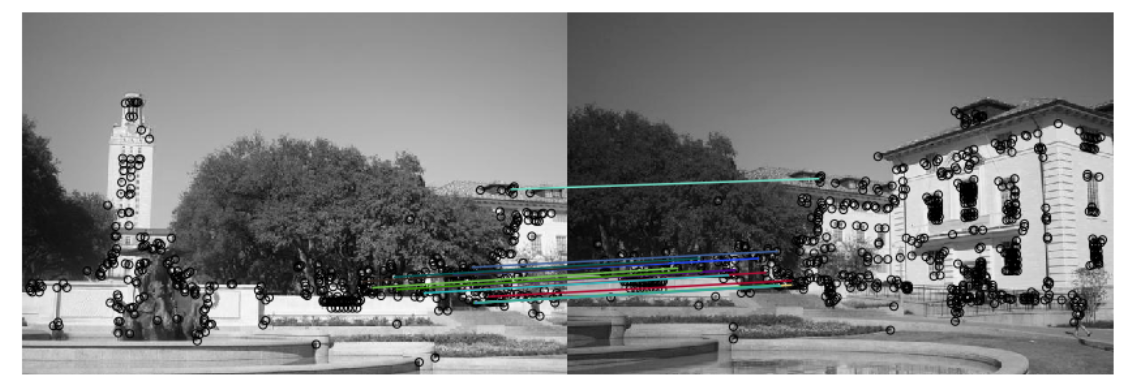
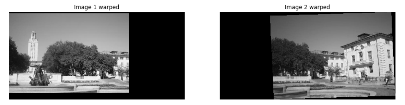
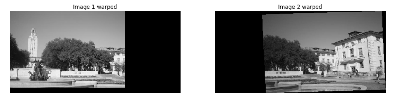
现在，我们可以利用新计算的到的转换矩阵 $H$ 来生成一张更稳定的全景图像了。

output_shape, offset = get_output_space(img1, [img2], [H])

# 进行坐标变换
img1_warped = warp_image(img1, np.eye(3), output_shape, offset)# 图片1不变，因此用单位阵作为变换矩阵
img1_mask = (img1_warped != -1) # Mask不等于-1表示该位置为原图片插值后的点
img1_warped[~img1_mask] = 0     # Mask取反表示在该位置没有值（该位置为背景），置0使得该位置变黑

img2_warped = warp_image(img2, H, output_shape, offset)
img2_mask = (img2_warped != -1) # Mask不等于-1表示该位置为原图片插值后的点
img2_warped[~img2_mask] = 0     # Mask取反表示在该位置没有值（该位置为背景），置0使得该位置变黑

# 显示坐标变换后的图片
plt.subplot(1,2,1)
plt.imshow(img1_warped)
plt.title('Image 1 warped')
plt.axis('off')

plt.subplot(1,2,2)
plt.imshow(img2_warped)
plt.title('Image 2 warped')
plt.axis('off')

plt.show()

merged = img1_warped + img2_warped

# 确定哪些值被加了两次
overlap = (img1_mask * 1.0 +  # bool 型转成 float 
           img2_mask)

# 重合部分的值除以2，未重合的部分除以1，以保证亮度一致
normalized = merged / np.maximum(overlap, 1)
plt.imshow(normalized)
plt.axis('off')
plt.show()

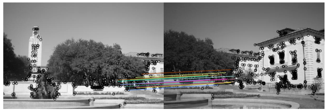
这个结果就是我们所希望的结果了，虽然在边缘处过渡不够平滑，但是非常不错的实现了图像的变形与配准。

7.2 梯度方向直方图部分

在前面的计算中，我们利用simple_descriptor来计算特征点的特征向量。但在这一模块里，我们将会利用HOG来计算特征点的特征。

HOG 值得是梯度方向直方图。在HOG算法中,我们利用梯度的方向分布来当做特征向量。梯度（x和y方向）在一幅图片中是很有用的，我们可以利用它的大小来判断点的类型，例如边缘等。

HOG的步骤包括:

计算x和y方向的梯度图像
计算梯度直方图：将图片分成若干个cell，并对每个cell计算梯度直方图
将若干个cell合成一个block，并将里面的梯度直方图转成特征向量
将特征向量归一化

from panorama import hog_descriptor

img1 = imread('uttower1.jpg', as_grey=True)
img2 = imread('uttower2.jpg', as_grey=True)

# 关键点检测
keypoints1 = corner_peaks(harris_corners(img1, window_size=3),
                          threshold_rel=0.05,
                          exclude_border=8)
keypoints2 = corner_peaks(harris_corners(img2, window_size=3),
                          threshold_rel=0.05,
                          exclude_border=8)

# 提取特征
desc1 = describe_keypoints(img1, keypoints1,
                           desc_func=hog_descriptor,
                           patch_size=16)
desc2 = describe_keypoints(img2, keypoints2,
                           desc_func=hog_descriptor,
                           patch_size=16)

# 特征匹配
matches = match_descriptors(desc1, desc2, 0.7)

# 画出匹配的特征
fig, ax = plt.subplots(1, 1, figsize=(15, 12))
ax.axis('off')
plot_matches(ax, img1, img2, keypoints1, keypoints2, matches)
plt.show()

一旦我们使用HOG描述算法完成了对特征点的描述，我们就能通过计算特征点之间的距离完成特征点之间的匹配。随后，我们可以利用RANSAC算法来进一步挑选稳定的匹配对(robust matches)，从而计算出准确的转换方程。

from panorama import ransac

# 设置相同的seed以保证生成的随机数相同
np.random.seed(131)

H, robust_matches = ransac(keypoints1, keypoints2, matches, threshold=1)

# 画出匹配的点
fig, ax = plt.subplots(1, 1, figsize=(15, 12))
plot_matches(ax, img1, img2, keypoints1, keypoints2, robust_matches)
plt.axis('off')
plt.show()

plt.imshow(imread('solution_hog_ransac.png'))
plt.axis('off')
plt.title('HOG descriptor + RANSAC Solution')
plt.show()

output_shape, offset = get_output_space(img1, [img2], [H])

# 坐标变换
img1_warped = warp_image(img1, np.eye(3), output_shape, offset)# 图片1只需要平移，因此用单位阵作为变换矩阵
img1_mask = (img1_warped != -1) # Mask不等于-1表示该位置为原图片插值后的点
img1_warped[~img1_mask] = 0     # Mask取反表示在该位置没有值（该位置为背景），置0使得该位置变黑

img2_warped = warp_image(img2, H, output_shape, offset)
img2_mask = (img2_warped != -1) # Mask不等于-1表示该位置为原图片插值后的点
img2_warped[~img2_mask] = 0     # Mask取反表示在该位置没有值（该位置为背景），置0使得该位置变黑

# 画出坐标变换后的图像
plt.subplot(1,2,1)
plt.imshow(img1_warped)
plt.title('Image 1 warped')
plt.axis('off')

plt.subplot(1,2,2)
plt.imshow(img2_warped)
plt.title('Image 2 warped')
plt.axis('off')

plt.show()

merged = img1_warped + img2_warped

# 确定哪些值被加了两次
overlap = (img1_mask * 1.0 +  # bool 型转成 float 
           img2_mask)

# 重合部分的值除以2，未重合的部分除以1，以保证亮度一致
normalized = merged / np.maximum(overlap, 1)
plt.imshow(normalized)
plt.axis('off')
plt.show()

plt.imshow(imread('solution_hog_panorama.png'))
plt.axis('off')
plt.title('HOG Descriptor Panorama Solution')
plt.show()

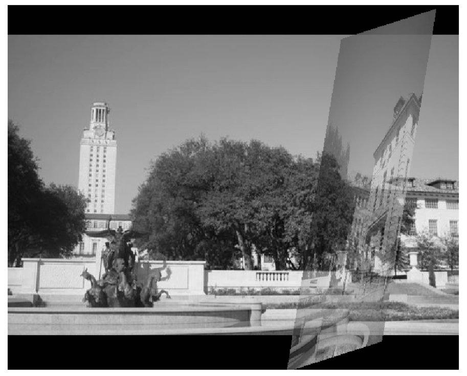
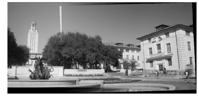
在该测试图像上，HOG的配准结果与Harris角点检测非常相似。

7.3 简单的图片融合策略

可以发现，在最终的输出图片里，融合区域存在明显的分界线。这些分界线并不是我们想要的，因此需要把它们去掉，其中有一个非常简单的方法叫做线性融合（linear blending）。

在前面计算融合图片的时候，我们将重合区域的强度值除以了2，其他部分除以1。这其实表示的是左右两张图片的比重相同（equally weighted）。但实际上，重合区域左右两边的比重并不应该相同：靠近左边图片的部分，左边图片的比重应该更大；靠近右边图片的部分，右边图片的比重应该更大。据此，我们可以利用线性融合的方法来提升最终全景图片的质量。

线性融合可以用以下几步进行实现:

确定融合区域的左边界和右边界；
给图片1确定一个权重矩阵:
- 从图片1的最左边到融合区域的最左边，weight为1；
- 从融合区域的最左边到图片1的最右边，weight从1到0进行分布；
给图片2确定一个权重矩阵:
- 从融合区域的最右边到图片2的最右边，weight为1；
- 从融合区域的最左边到图片1的最右边，weight从0到1进行分布；
分别对左右两张图片应用权重矩阵；
将两张图相加。

from panorama import linear_blend

img1 = imread('uttower1.jpg', as_grey=True)
img2 = imread('uttower2.jpg', as_grey=True)

# 设置相同的seed以保证生成的随机数相同
np.random.seed(131)

# 检测特征点
keypoints1 = corner_peaks(harris_corners(img1, window_size=3),
                          threshold_rel=0.05,
                          exclude_border=8)
keypoints2 = corner_peaks(harris_corners(img2, window_size=3),
                          threshold_rel=0.05,
                          exclude_border=8)

# 提取特征描述向量
desc1 = describe_keypoints(img1, keypoints1,
                           desc_func=hog_descriptor,
                           patch_size=16)
desc2 = describe_keypoints(img2, keypoints2,
                           desc_func=hog_descriptor,
                           patch_size=16)

# 进行特征描述向量的匹配
matches = match_descriptors(desc1, desc2, 0.7)

H, robust_matches = ransac(keypoints1, keypoints2, matches, threshold=1)

output_shape, offset = get_output_space(img1, [img2], [H])

# 将图片放到最终输出图里面
img1_warped = warp_image(img1, np.eye(3), output_shape, offset)
img1_mask = (img1_warped != -1) # Mask == 1 inside the image
img1_warped[~img1_mask] = 0     # Return background values to 0

img2_warped = warp_image(img2, H, output_shape, offset)
img2_mask = (img2_warped != -1) # Mask == 1 inside the image
img2_warped[~img2_mask] = 0     # Return background values to 0

# 将两张图片拼成一张
merged = linear_blend(img1_warped, img2_warped)

plt.imshow(merged)
plt.axis('off')
plt.show()

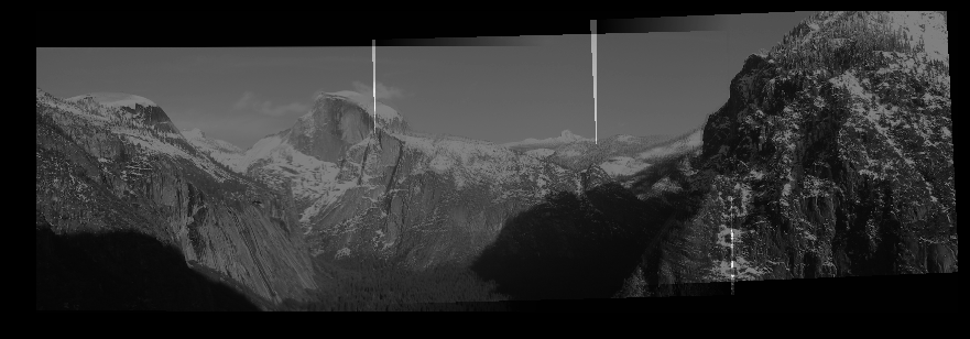
7.4 多图像的配准——全景图像拼接

假设现在你有 $m$ 张图片 $(I_1,I_2,...,I_m$ ,我们可以把相邻的两张图片当成一组，然后计算图片 $I_{i+1}$ 到图片 $I_i$ 的坐标转换矩阵，也就是前面我们所完成的affine变换矩阵。接着，我们可以选择最中间的一张照片作为参考图片(reference image $I_{ref}$ )，并将其他照片的坐标系统转换到该图片中来，从而完成 $m$ 张图片的拼接。

from panorama import stitch_multiple_images

# 设置相同的seed以保证生成的随机数相同
np.random.seed(131)

# 载入需要进行拼接的图片
img1 = imread('yosemite1.jpg', as_grey=True)
img2 = imread('yosemite2.jpg', as_grey=True)
img3 = imread('yosemite3.jpg', as_grey=True)
img4 = imread('yosemite4.jpg', as_grey=True)

imgs = [img1, img2, img3, img4]

# 将图片拼接到一起
panorama = stitch_multiple_images(imgs, desc_func=simple_descriptor, patch_size=5)

# 显示拼接后的图片
plt.imshow(panorama)
plt.axis('off')
plt.show()

7.5 拓展讨论

本文的代码为了减少计算量，是对灰度图像进行处理的，但这并不意味着不能对彩色图像进行特征提取与拼接。计算特征并基于特征配准，这对于彩色图像而言其实同样可行，基于灰度图像的特征或综合三通道的图像进行特征匹配，都可以并实现彩色图像上的拼接。

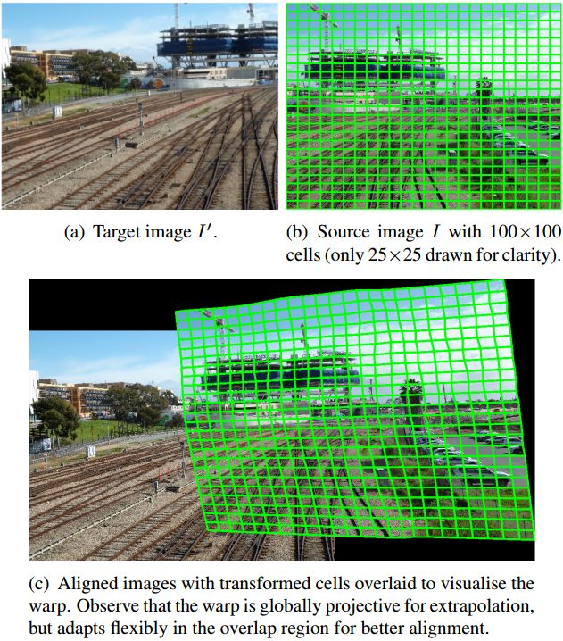
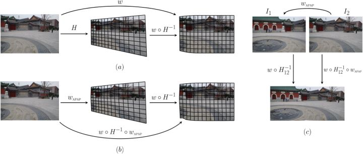
此外，在了解图像拼接领域的相关研究中，有3到4种主流的图像拼接方向，其中非常有意思的一种是基于网格变形的图像拼接（Shape-Preserving Half-Projective(SPHP)，2014CVPR），其方法是求解一个最优的公共平面将所有图像映射到公共平面上。

SPHP从形状矫正的角度出发，非重叠区域逐渐过渡到全局相似，并对整个图像增加相似变换约束，矫正拼接图像的形状，减少投影失真（算法的核心思想——网格变形，如下图)

算法流程图如下：

其Matlab代码可以在该网址下载：www.cmlab.csie.ntu.edu.tw/~frank/SPH/cvpr14_SPHP_code.tar

该方法的特征点匹配结果：

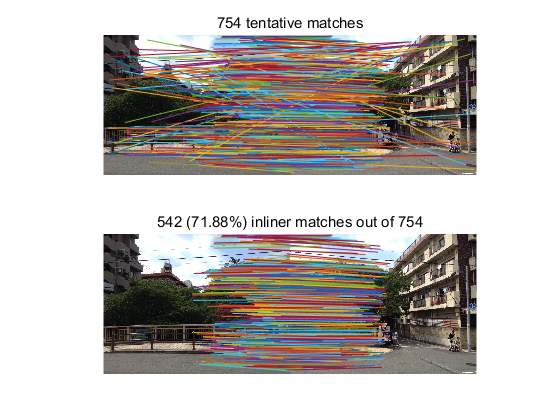
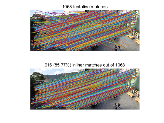
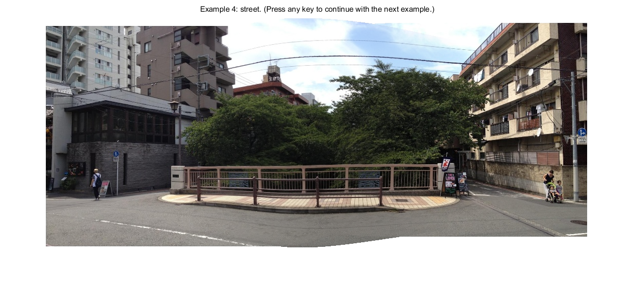
该方法的拼接结果有非常好的效果，可以做到对图像局部非线性畸变的矫正，这是网格变形的优势所在。

有兴趣的朋友可以自行了解该领域的相关方法，特征与配准目前仍是计算机视觉领域的热点研究方向。

8 写在最后

Harris角点检测的参考文献，1988发表，被引用次数17316

[1] Harris C G, Stephens M. A combined corner and edge detector[C]//Alvey vision conference. 1988, 15(50): 10-5244.

谷歌学术和百度学术都没法看这篇88年的文章的原文，估计有点老了....放个某国内文档网的在线浏览页面吧 max.book118.com/html/2017/0…

方向梯度直方图的参考文献，IJCV和CVPR都是计算机视觉三大顶会之一，[2]2005年发表，被引用次数30607，[3]2012年发表，被引166

[2] Dalal N , Triggs B . Histograms of Oriented Gradients for Human Detection[C]// 2005 IEEE Computer Society Conference on Computer Vision and Pattern Recognition (CVPR'05). IEEE, 2005.

eee.uci.edu/16w/34830/h…

[3] Chandrasekhar V , Takacs G , Chen D M , et al. Compressed Histogram of Gradients: A Low-Bitrate Descriptor[J]. International Journal of Computer Vision, 2012, 96(3):384-399.

web.stanford.edu/~bgirod/pdf…

SPHP图像拼接，2014年发表，被引量158：

[4] Chang C H, Sato Y, Chuang Y Y. Shape-preserving half-projective warps for image stitching[C]//Proceedings of the IEEE Conference on Computer Vision and Pattern Recognition. 2014: 3254-3261.