

- 原文地址:How to easily Detect Objects with Deep Learning on Raspberry Pi
- 原文作者:Sarthak Jain
- 译文出自:掘金翻译计划
- 本文永久链接:github.com/xitu/gold-m…
- 译者:Starrier
- 校对者:luochen1992、jasonxia23
真实世界带来的挑战,是有限的数据以及小型硬件,诸如手机和树莓派等,这些硬件无法运行复杂的深度学习模型。这篇文章演示了如何使用树莓派进行对象检测,就像公路上的汽车,冰箱里的橘子,文件上的签名,太空中的特斯拉。
免责声明:我正在用更少的数据和无硬件的方式构建 nanonets.com 来帮助建立机器学习。
如果你没有耐心继续阅读下去,可以直接翻阅到底部查看 Github 的仓库。
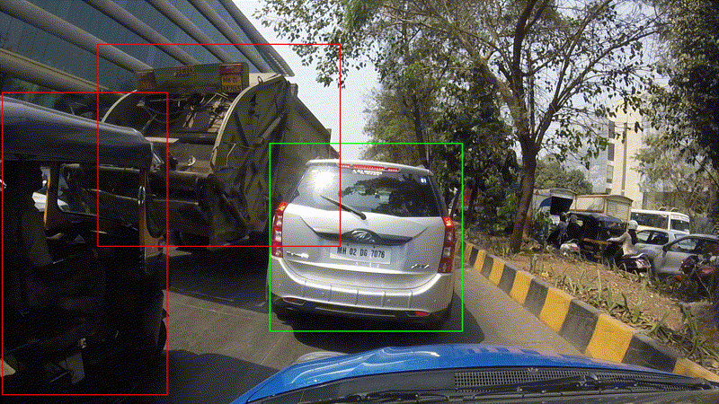
检测孟买路上的车辆。
为什么要检测对象?为什么使用树莓派?
树莓派是一款优秀的硬件,它已经捕获了与售卖 1500 万台设备同时代的人的心,甚至于黑客用其构建了更酷的项目。鉴于深度学习和树莓派相机的流行,我们认为如果能够通过树莓派进行深度学习来检测任何对象,会是一件非常有意义的事情。
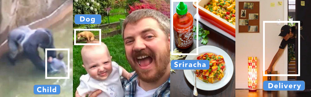
现在你将能够在你的自拍中发现一个 potobomber,有人进入 Harambe 的笼子,在那里有人让 Sriracha 或 Amazon 送货员进入你的房子。
什么是对象检测?
20M 年的进化使人类的视觉得到了相当大的进化。人类大脑有 30% 的神经元负责处理视觉(相比之下,触觉和听觉分别为 8% 和 3%)。与机器相比,人类有两大优势。一是立体视觉,二是近乎无限的训练数据(一个 5 岁的婴儿,以 30fps 的速度获取大约 2.7B 的图像)。
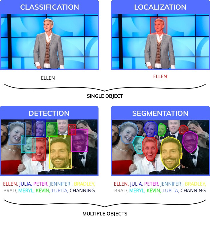
为了模仿人类层次的表现水平,科学家将视觉感知任务分解为四个不同的类别。
- 分类,为整个图像指定一个标签
- Localization,为特定标签指定一个边框
- 对象检测,在图像中绘制多个边界框
- 图像分割,创建图像中物体所在位置的精确部分
对于各种应用来说,对象检测已经足够好了(即使图像分割结果更为精确,但它受到创建训练数据的复杂性影响。对于一个人类标注者来说,分割图像所花的时间比绘制边界框要多 12 倍;这是更多的轶事,但缺乏一个来源)。而且在检测对象之后,可以单独从边界框中分割对象。
使用对象检测:
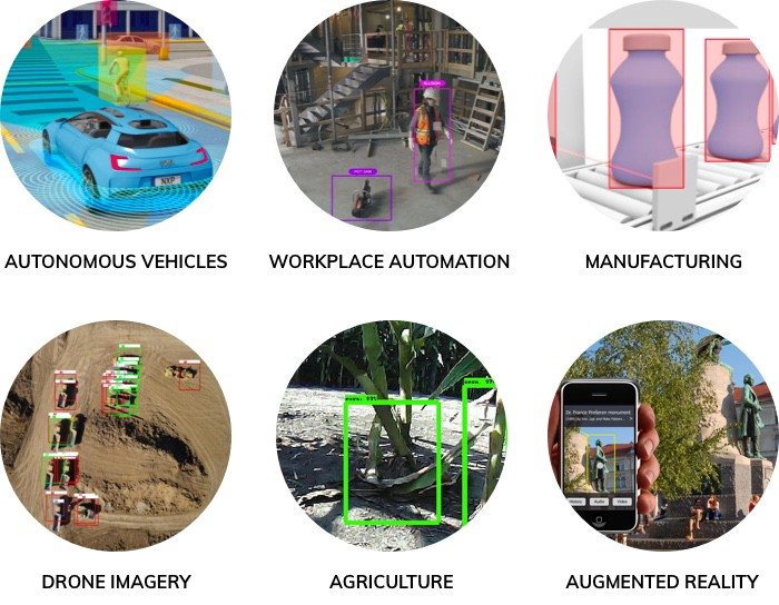
对象检测具有重要的现实意义,已经在各行业中被广泛使用。以下是相关示例:
我如何使用对象检测来解决我自己的问题?
对象检测可用来回答各种问题。这是粗略的分类:
- 在我的图像中是否存在对象?例如,我家有入侵者么。
- 对象在哪里,在图像中?例如,当一辆汽车试图在世界各地行驶时,知道物体在哪里是很重要的。
- 有多少个对象,它们都在图像中么? 对象检测是计算物体的最有效的方法之一。例如,一个仓库里的架子上有多少箱子。
- 什么是不同类型的对象在图像中?比如哪个动物在动物园的哪个地方?
- 对象的大小是多少? 尤其是使用静态相机时,很容易计算出物体的大小。比如芒果的大小是多少?
- **不同对象如何相互作用?**足球场上的阵型如何影响结果?
- 与时间有关的对象在何处(追踪对象)比如追踪像火车这样的移动物体,并计算它的速度等。
20 行以下代码中的对象检测
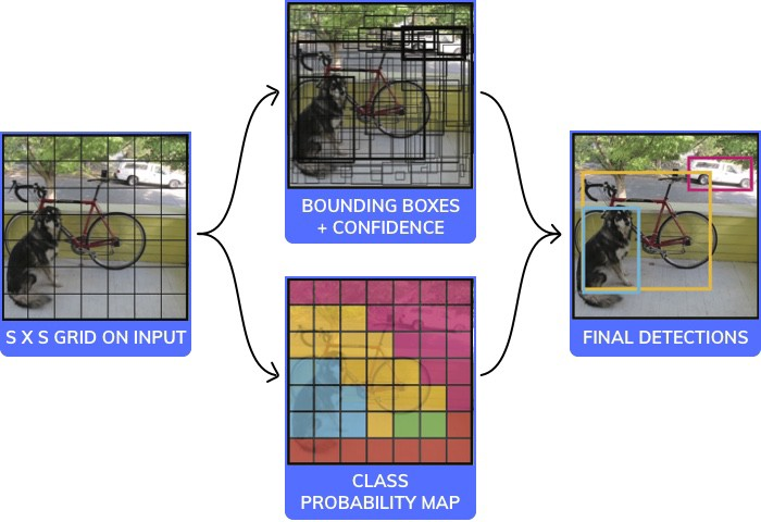
YOLO 算法可视化。
有多种用于对象检测的模型/体系结构。在速度、尺寸和精度之间进行权衡。我们选了一个最受欢迎的:YOLO(您只看了一次)。并在 20 行以下的代码中展示了它的工作原理(如果忽略注释的 haunted)。
注意:这是伪代码,不会成为一个有用的例子。它有一个接近 CNN 标准的部分黑盒,如下所示。
你可以在这里阅读全文:pjreddie.com/media/files…
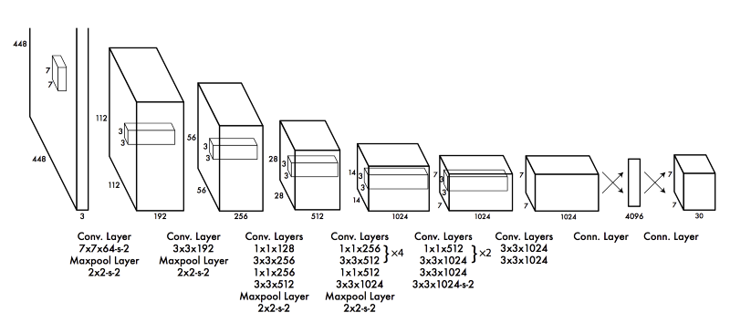
YOLO 中的卷积神经网络结构。
#this is an Image of size 140x140. We will assume it to be black and white (ie only one channel, it would have been 140x140x3 for rgb)
image = readImage()

#We will break the Image into 7 coloumns and 7 rows and process each of the 49 different parts independently
NoOfCells = 7

#we will try and predict if an image is a dog, cat, cow or wolf. Therfore the number of classes is 4
NoOfClasses = 4
threshold = 0.7

#step will be the size of step to take when moving across the image. Since the image has 7 cells step will be 140/7 = 20
step = height(image)/NoOfCells

#stores the class for each of the 49 cells, each cell will have 4 values which correspond to the probability of a cell being 1 of the 4 classes
#prediction_class_array[i,j] is a vector of size 4 which would look like [0.5 #cat, 0.3 #dog, 0.1 #wolf, 0.2 #cow]
prediction_class_array = new_array(size(NoOfCells,NoOfCells,NoOfClasses))

#stores 2 bounding box suggestions for each of the 49 cells, each cell will have 2 bounding boxes, with each bounding box having x, y, w ,h and c predictions. (x,y) are the coordinates of the center of the box, (w,h) are it's height and width and c is it's confidence
predictions_bounding_box_array = new_array(size(NoOfCells,NoOfCells,NoOfCells,NoOfCells))

#it's a blank array in which we will add the final list of predictions
final_predictions = []

#minimum confidence level we require to make a prediction
threshold = 0.7

for (i<0; i<NoOfCells; i=i+1):
	for (j<0; j<NoOfCells;j=j+1):
		#we will get each "cell" of size 20x20, 140(image height)/7(no of rows)=20 (step) (size of each cell)"
		#each cell will be of size (step, step)
		cell = image(i:i+step,j:j+step)

		#we will first make a prediction on each cell as to what is the probability of it being one of cat, dog, cow, wolf
		#prediction_class_array[i,j] is a vector of size 4 which would look like [0.5 #cat, 0.3 #dog, 0.1 #wolf, 0.2 #cow]
		#sum(prediction_class_array[i,j]) = 1
		#this gives us our preidction as to what each of the different 49 cells are
		#class predictor is a neural network that has 9 convolutional layers that make a final prediction
		prediction_class_array[i,j] = class_predictor(cell)

		#predictions_bounding_box_array is an array of 2 bounding boxes made for each cell
		#size(predictions_bounding_box_array[i,j]) is [2,5]
		#predictions_bounding_box_array[i,j,1] is bounding box1, predictions_bounding_box_array[i,j,2] is bounding box 2
		#predictions_bounding_box_array[i,j,1] has 5 values for the bounding box [x,y,w,h,c]
		#the values are x, y (coordinates of the center of the bounding box) which are whithin the bounding box (values ranging between 0-20 in your case)
		#the values are h, w (height and width of the bounding box) they extend outside the cell and are in the range of [0-140]
		#the value is c a confidence of overlap with an acutal bounding box that should be predicted
		predictions_bounding_box_array[i,j] = bounding_box_predictor(cell)

		#predictions_bounding_box_array[i,j,0, 4] is the confidence value for the first bounding box prediction
		best_bounding_box =  [0 if predictions_bounding_box_array[i,j,0, 4] > predictions_bounding_box_array[i,j,1, 4] else 1]

		# we will get the class which has the highest probability, for [0.5 #cat, 0.3 #dog, 0.1 #wolf, 0.2 #cow], 0.5 is the highest probability corresponding to cat which is at position 0. So index_of_max_value will return 0
		predicted_class = index_of_max_value(prediction_class_array[i,j])

		#we will check if the prediction is above a certain threshold (could be something like 0.7)
		if predictions_bounding_box_array[i,j,best_bounding_box, 4] * max_value(prediction_class_array[i,j]) > threshold:

			#the prediction is an array which has the x,y coordinate of the box, the height and the width
			prediction = [predictions_bounding_box_array[i,j,best_bounding_box, 0:4], predicted_class]

			final_predictions.append(prediction)


print final_predictions
YOLO 在 <20 行代码中的解释。
我们如何构建用于对象检测的深度学习模型?
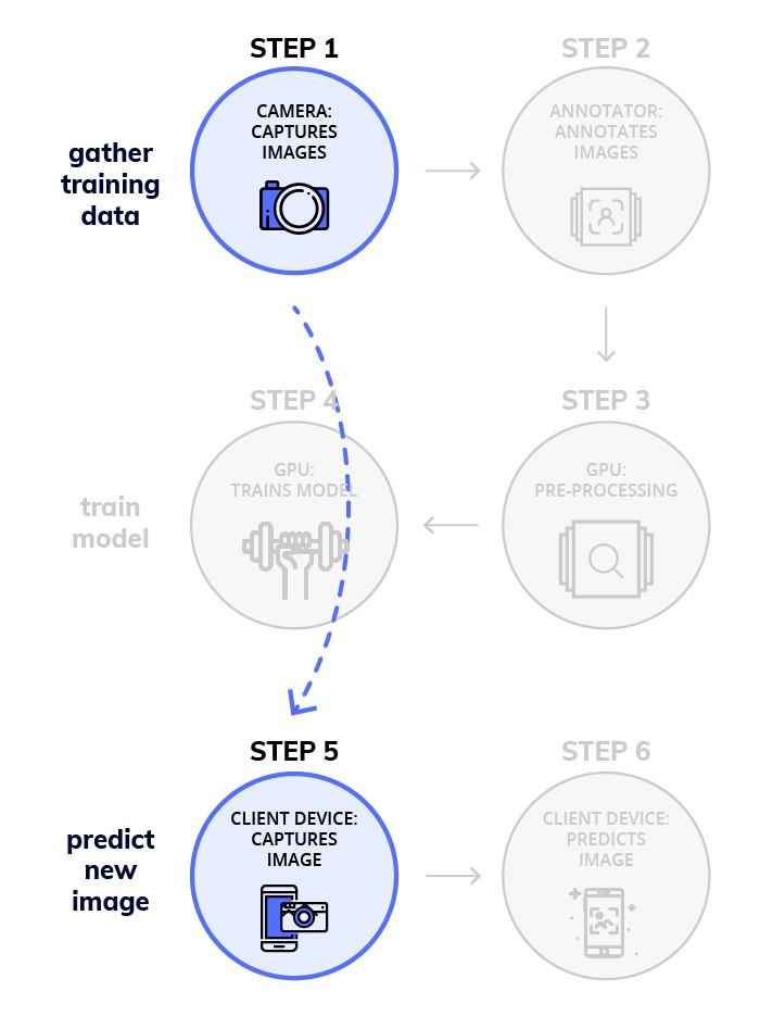
深度学习工作流的 6 个主要步骤将分成 3 个阶段
- 收集训练数据
- 训练模型
- 预测新图像
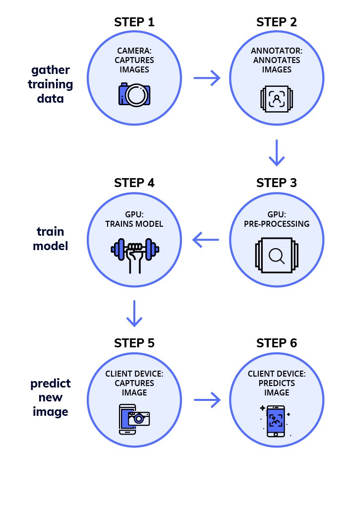
阶段 1 —— 收集训练数据
第 1 步 收集图像(每个对象至少有 100 张图像):
在这个任务中,每个对象需要几百张图像。尝试将数据捕获到您最终要对其进行预测的数据上。
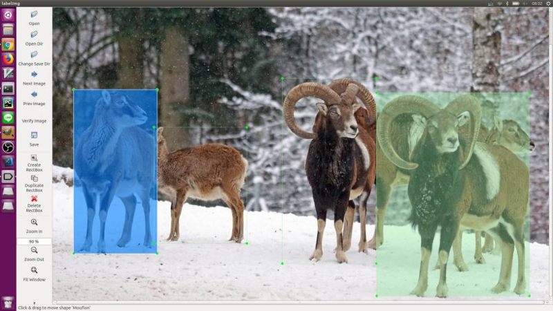
第 2 步 注解(手动绘制这些图像):
在图像上绘制边界框。您可以使用像 labelImg 这样的工具。您需要一些人来注释您的图像。这是一个相当密集且耗时的任务。
阶段 2 — 在 GPU 机器上训练模型
第 3 步 寻找可以迁移学习的预训练模型
您可以在 medium.com/nanonets/na… 中阅读到更多有关这方面的信息。您需要一个预训练模型,这样您就可以减少训练所需的数据量。没有它,您可能需要几十万张的图像来训练模型。
第 4 步骤, 在 GPU 上训练(像 AWS/GCP 等云服务或您自己的 GPU 机器):
Docker 镜像
训练模型的过程不是必要的,但创建 docker 镜像使得训练变得更加简单的过程很难简化。
你可以通过运行如下内容来开始训练模型:
sudo nvidia-docker run -p 8000:8000 -v `pwd`:data docker.nanonets.com/pi_training -m train -a ssd_mobilenet_v1_coco -e ssd_mobilenet_v1_coco_0 -p '{"batch_size":8,"learning_rate":0.003}'
有关如何使用的详细信息,请参阅此链接
docker 镜像拥有一个可以用以下参数调用的 run.sh 脚本
run.sh [-m mode] [-a architecture] [-h help] [-e experiment_id] [-c checkpoint] [-p hyperparameters]

-h          display this help and exit
-m          mode: should be either `train` or `export`
-p          key value pairs of hyperparameters as json string
-e          experiment id. Used as path inside data folder to run current experiment
-c          applicable when mode is export, used to specify checkpoint to use for export
您可以在以下找到更多细节:
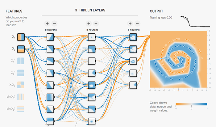
为了训练模型,您需要选择正确的超参数。
找到正确的参数
“深度学习”的艺术含有一点点讽刺,但它会尝试找出哪些会为您的模型获得最高精度的最佳参数。与此相关的是某些程度的黑魔法以及一点理论。这是找到正确参数的好资源。
量化模型(使其更小以适应像树莓派或手机这样的小型设备)
诸如手机和树莓派这样的小型设备,内存和计算能力都很小。
训练神经网络是通过对权重施加许多微小推进完成的,而这些微小的增量通常需要浮点精度才能工作(尽管这里也有研究努力使用量化表示)。
采用预先训练模型并运行推理是非常不同的。深度神经网络的神奇特性之一是,它们往往能很好地处理输入中的高噪声。
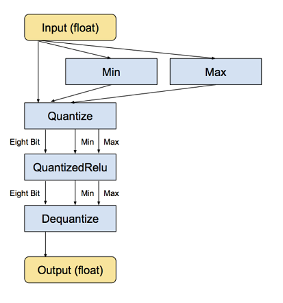
为什么要量化?
例如,神经网络模型会占用大量磁盘空间,起初 AlexNet 是 200 MB 以上的浮点格式。因为在单个模型中经常有数百万个神经连接,因此几乎所有大小都被神经连接的权重所决定。
神经网络的节点和权重起初被存储为 32-bit 浮点数,最简单的量化动机是通过存储每个层的最小和最大值来缩小文件大小,然后将每个浮点值压缩为一个 8 位整数,文件大小因此减小了 75%。
量化代码:
curl -L "https://storage.googleapis.com/download.tensorflow.org/models/inception_v3_2016_08_28_frozen.pb.tar.gz" |
  tar -C tensorflow/examples/label_image/data -xz
bazel build tensorflow/tools/graph_transforms:transform_graph
bazel-bin/tensorflow/tools/graph_transforms/transform_graph \
--in_graph=tensorflow/examples/label_image/data/inception_v3_2016_08_28_frozen.pb \
  --out_graph=/tmp/quantized_graph.pb \
  --inputs=input \
  --outputs=InceptionV3/Predictions/Reshape_1 \
  --transforms='add_default_attributes strip_unused_nodes(type=float, shape="1,299,299,3")
    remove_nodes(op=Identity, op=CheckNumerics) fold_constants(ignore_errors=true)
    fold_batch_norms fold_old_batch_norms quantize_weights quantize_nodes
    strip_unused_nodes sort_by_execution_order
第 3 阶段:使用树莓派预测新图像
第 5 步,通过相机捕捉新图像
你需要树莓派生活和工作。然后捕获一个新图像
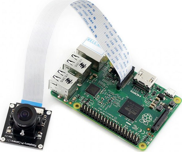
安装说明参见此链接
import picamera, os
from PIL import Image, ImageDraw
camera = picamera.PiCamera()
camera.capture('image1.jpg')
os.system("xdg-open image1.jpg")
捕获新图像的代码。
第 6 步,预测新图像
下载模型
一旦你完成了模型的训练,你就可以把它下载到你的树莓派上了。要导出模型运行:
sudo nvidia-docker run -v `pwd`:data docker.nanonets.com/pi_training -m export -a ssd_mobilenet_v1_coco -e ssd_mobilenet_v1_coco_0 -c /data/0/model.ckpt-8998
然后将模型下载到树莓派上。
在树莓派上下载 Tensorflow
根据设备的不同,您可能需要稍微更改安装
sudo apt-get install libblas-dev liblapack-dev python-dev libatlas-base-dev gfortran python-setuptools libjpeg-dev

sudo pip install Pillow

sudo pip install http://ci.tensorflow.org/view/Nightly/job/nightly-pi-zero/lastSuccessfulBuild/artifact/output-artifacts/tensorflow-1.4.0-cp27-none-any.whl

git clone [https://github.com/tensorflow/models.git](https://github.com/tensorflow/models.git)

sudo apt-get install -y protobuf-compiler

cd models/research/protoc object_detection/protos/*.proto --python_out=.

export PYTHONPATH=$PYTHONPATH:/home/pi/models/research:/home/pi/models/research/slim
运行模型以预测新图像
python ObjectDetectionPredict.py --model data/0/quantized_graph.pb --labels data/label_map.pbtxt --images /data/image1.jpg /data/image2.jpg
树莓派的性能基准测试
树莓派对内存和计算都有限制(与树莓派 GPU 兼容的 Tensorflow 版本仍然不可用)。因此,对基准测试来说,每个模型需要多少时间才能对新图像进行预测非常重要。
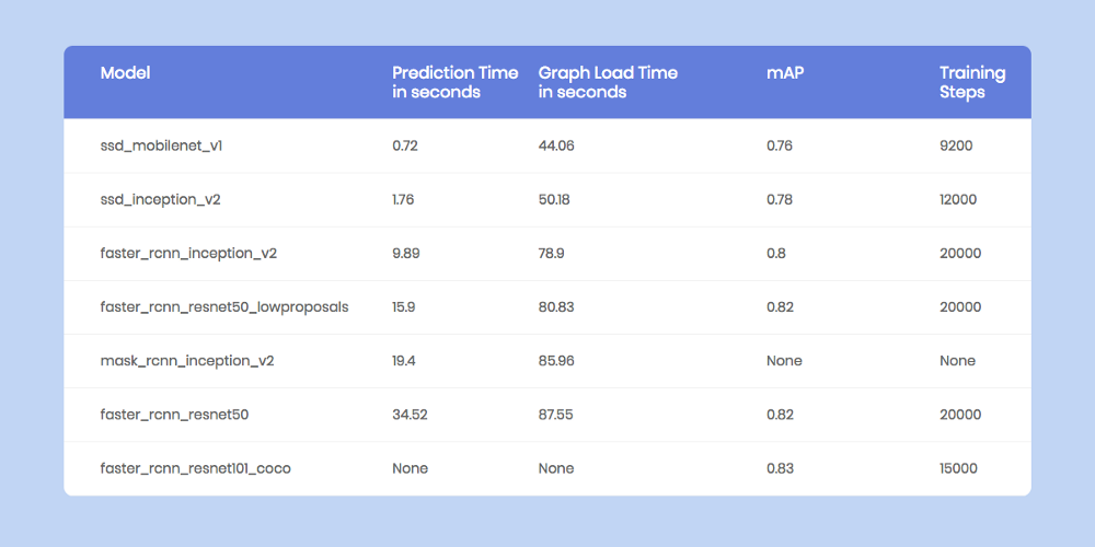
在树莓派中运行不同对象检测的基准测试。
我们在 NanoNets 的目标是使深度学习工作更加简单。对象检测是我们关注的一个主要领域,我们已经制定了一个工作流来解决实现深度学习模型的许多挑战。
NanoNets 如何使过程更简单:
1. 无需注解
我们已经删除了注释图像的需求,我们有专业的注释人员为为您的图像注释。
2. 自动优化模型与超参数的选择
我们为您自动化训练最好的模型。为了实现这个,我们运行一组具有不同参数的模型,来为您的数据选择最佳模型。
3. 不需要昂贵的硬件和 GPU
NanoNets 完全在云端运行而且无需任何硬件。这使得它更容易使用。
4. 适合像树莓派这样的移动设备
因为像树莓派和手机这样的设备并不是为了运行复杂的计算任务而构建的,所以您可以把工作量外包给我们的云,它会为您完成所有的计算
这里是使用 NanoNets API 对图像进行预测的简单片段
import picamera, json, requests, os, random
from time import sleep
from PIL import Image, ImageDraw

#capture an image
camera = picamera.PiCamera()
camera.capture('image1.jpg')
print('caputred image')

#make a prediction on the image
url = 'https://app.nanonets.com/api/v2/ObjectDetection/LabelFile/'
data = {'file': open('image1.jpg', 'rb'), \
    'modelId': ('', 'YOUR_MODEL_ID')}
response = requests.post(url, auth=requests.auth.HTTPBasicAuth('YOUR_API_KEY', ''), files=data)
print(response.text)

#draw boxes on the image
response = json.loads(response.text)
im = Image.open("image1.jpg")
draw = ImageDraw.Draw(im, mode="RGBA")
prediction = response["result"][0]["prediction"]
for i in prediction:
    draw.rectangle((i["xmin"],i["ymin"], i["xmax"],i["ymax"]), fill=(random.randint(1, 255),random.randint(1, 255),random.randint(1, 255),127))
im.save("image2.jpg")
os.system("xdg-open image2.jpg")
使用 NanoNets 对新图像进行预测的代码
构建您自己的 NanoNet
您可以尝试从以下几点来构建属于自己的模型:
1. 使用 GUI(也可以自动注释图像):nanonets.com/objectdetec…
2. 使用我们的 API:github.com/NanoNets/ob…
第 1 步:克隆仓库
git clone [https://github.com/NanoNets/object-detection-sample-python.git](https://github.com/NanoNets/object-detection-sample-python.git)
cd object-detection-sample-python
sudo pip install requests
第 2 步:获取您的免费 API 的密钥
从 app.nanonets.com/user/api_ke… 中获取您的免费 API 密钥
第 3 步:将 API 密钥设置为环境变量
export NANONETS_API_KEY=YOUR_API_KEY_GOES_HERE
第 4 步:创建新模型
python ./code/create-model.py
注意:这将生成下一步所需的模型 ID
第 5 步:添加模型 ID 作为环境变量
export NANONETS_MODEL_ID=YOUR_MODEL_ID
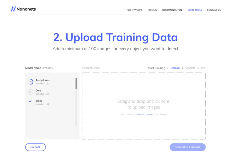
第 6 步:上传训练数据
收集您想要检测对象的图像。您可以使用我们的 web UI(https://app.nanonets.com/ObjectAnnotation/?appId=YOUR_MODEL_ID) 对其进行注释,或者使用像 labelImg 这样的开源工具。一旦在文件夹中准备好数据集,images(图像文件)和 annotations(图像文件注解),就可以开始上传数据集了。
python ./code/upload-training.py
第 7 步:训练模型
一旦图像上传完毕,就开始训练模型
python ./code/train-model.py
第 8 步:获取模型状态
模型训练需要 2 个小时。一旦模型被训练,您将收到一封电子邮件。同时检查模型的状态
watch -n 100 python ./code/model-state.py
第 9 步:预测
一旦模型训练好了,您就可以使用来进行预测
python ./code/prediction.py PATH_TO_YOUR_IMAGE.jpg
代码(GitHub 仓库)
训练模型的 Github 仓库:
为树莓派做出预测的 GitHub 仓库(即检测新对象):
带有注释的数据集:
掘金翻译计划 是一个翻译优质互联网技术文章的社区,文章来源为 掘金 上的英文分享文章。内容覆盖 Android、iOS、前端、后端、区块链、产品、设计、人工智能等领域,想要查看更多优质译文请持续关注 掘金翻译计划、官方微博、知乎专栏。
