相关文章目录:
- 机器学习 之线性回归
- 机器学习 之逻辑回归及python实现
- 机器学习项目实战 交易数据异常检测
- 机器学习之 决策树(Decision Tree)
- 机器学习之 决策树(Decision Tree)python实现
- 机器学习之 PCA(主成分分析)
- 机器学习之 特征工程
现在有一批经过处理后的信用卡用户交易数据,我们需要通过这些数据学习一个模型,可以用来预测新的一条交易数据是否涉嫌信用卡欺诈。
首先,当然先需要导入下必要的python库
import pandas as pd
import matplotlib.pyplot as plt
import numpy as np

%matplotlib inline
先读取下原始数据看看
data = pd.read_csv("creditcard.csv")
print(data.shape)
data.head() #打印前5行
(284807, 31)
| Time | V1 | V2 | V3 | V4 | V5 | V6 | V7 | V8 | V9 | ... | V21 | V22 | V23 | V24 | V25 | V26 | V27 | V28 | Amount | Class | |
|---|---|---|---|---|---|---|---|---|---|---|---|---|---|---|---|---|---|---|---|---|---|
| 0 | 0.0 | -1.359807 | -0.072781 | 2.536347 | 1.378155 | -0.338321 | 0.462388 | 0.239599 | 0.098698 | 0.363787 | ... | -0.018307 | 0.277838 | -0.110474 | 0.066928 | 0.128539 | -0.189115 | 0.133558 | -0.021053 | 149.62 | 0 |
| 1 | 0.0 | 1.191857 | 0.266151 | 0.166480 | 0.448154 | 0.060018 | -0.082361 | -0.078803 | 0.085102 | -0.255425 | ... | -0.225775 | -0.638672 | 0.101288 | -0.339846 | 0.167170 | 0.125895 | -0.008983 | 0.014724 | 2.69 | 0 |
| 2 | 1.0 | -1.358354 | -1.340163 | 1.773209 | 0.379780 | -0.503198 | 1.800499 | 0.791461 | 0.247676 | -1.514654 | ... | 0.247998 | 0.771679 | 0.909412 | -0.689281 | -0.327642 | -0.139097 | -0.055353 | -0.059752 | 378.66 | 0 |
| 3 | 1.0 | -0.966272 | -0.185226 | 1.792993 | -0.863291 | -0.010309 | 1.247203 | 0.237609 | 0.377436 | -1.387024 | ... | -0.108300 | 0.005274 | -0.190321 | -1.175575 | 0.647376 | -0.221929 | 0.062723 | 0.061458 | 123.50 | 0 |
| 4 | 2.0 | -1.158233 | 0.877737 | 1.548718 | 0.403034 | -0.407193 | 0.095921 | 0.592941 | -0.270533 | 0.817739 | ... | -0.009431 | 0.798278 | -0.137458 | 0.141267 | -0.206010 | 0.502292 | 0.219422 | 0.215153 | 69.99 | 0 |
5 rows × 31 columns
可以看到,总共有284807个样本,每个样本有31个特征,其中V1到V28 这28个特征,是已经经过处理加密后的干净数据,虽然不知道具体代表什么意思,但是可以直接拿来用就可以了。剩下的几个特征,
Time表示交易时间
Amount 表示交易金额总量
Class 即输出,表示此条交易行为是否存在信用卡欺诈,0为正常,1为异常。 我们将Class为0的称为负样本,Class为1的称为正样本
特征缩放
另外,我们看下,Amount这个特征,和其他V1到V28特征相比,数值范围存在明显的差距,所以,我们需要对Amount 进行特征缩放
from sklearn.preprocessing import StandardScaler
# print(data['Amount'].reshape(-1,1))
data['normAmount'] = StandardScaler().fit_transform(data['Amount'].reshape(-1,1))
data = data.drop(['Time','Amount'],axis=1)  #删除不用的列
data.head()
| V1 | V2 | V3 | V4 | V5 | V6 | V7 | V8 | V9 | V10 | ... | V21 | V22 | V23 | V24 | V25 | V26 | V27 | V28 | Class | normAmount | |
|---|---|---|---|---|---|---|---|---|---|---|---|---|---|---|---|---|---|---|---|---|---|
| 0 | -1.359807 | -0.072781 | 2.536347 | 1.378155 | -0.338321 | 0.462388 | 0.239599 | 0.098698 | 0.363787 | 0.090794 | ... | -0.018307 | 0.277838 | -0.110474 | 0.066928 | 0.128539 | -0.189115 | 0.133558 | -0.021053 | 0 | 0.244964 |
| 1 | 1.191857 | 0.266151 | 0.166480 | 0.448154 | 0.060018 | -0.082361 | -0.078803 | 0.085102 | -0.255425 | -0.166974 | ... | -0.225775 | -0.638672 | 0.101288 | -0.339846 | 0.167170 | 0.125895 | -0.008983 | 0.014724 | 0 | -0.342475 |
| 2 | -1.358354 | -1.340163 | 1.773209 | 0.379780 | -0.503198 | 1.800499 | 0.791461 | 0.247676 | -1.514654 | 0.207643 | ... | 0.247998 | 0.771679 | 0.909412 | -0.689281 | -0.327642 | -0.139097 | -0.055353 | -0.059752 | 0 | 1.160686 |
| 3 | -0.966272 | -0.185226 | 1.792993 | -0.863291 | -0.010309 | 1.247203 | 0.237609 | 0.377436 | -1.387024 | -0.054952 | ... | -0.108300 | 0.005274 | -0.190321 | -1.175575 | 0.647376 | -0.221929 | 0.062723 | 0.061458 | 0 | 0.140534 |
| 4 | -1.158233 | 0.877737 | 1.548718 | 0.403034 | -0.407193 | 0.095921 | 0.592941 | -0.270533 | 0.817739 | 0.753074 | ... | -0.009431 | 0.798278 | -0.137458 | 0.141267 | -0.206010 | 0.502292 | 0.219422 | 0.215153 | 0 | -0.073403 |
5 rows × 30 columns
类不平衡问题
接下来,我们看下当前样本中,负样本和正样本分别有多少个
count_class = pd.value_counts(data['Class'],sort=True).sort_index()
print(count_class)
0    284315
1       492
Name: Class, dtype: int64
我们发现,负样本有284315个,而正样本只有492个,存在严重的正负样本比例不平衡,也就是类不平衡问题。下面具体来说下。
类不平衡是说在训练分类器模型时,样本集中的类别分布不均匀,比如上面那个问题,284807个数据,理想情况下,应该是正负样本数量近似相等;而像上面正样本284315个,负样本只有492个,这个就存在严重的类不平衡问题。
为啥要避免这个问题呢?从训练模型的角度来说,如果某类的样本数量很少,那么这个类别锁提供的‘信息’就会很少,这样的化,就会导致我们的模型训练效果很差。
如何避免呢,常用的有两种方式来使得不同类别样本比例相对平衡
- 下采样: 对训练集里面样本数量较多的类别(多数类)进行欠采样,抛弃一些样本来缓解类不平衡。
- 过采样: 对训练集里面样本数量较少的类别(少数类)进行过采样,合成新的样本来缓解类不平衡。 这个时候会用到一个非常经典的过采样算法SMOTE
我们先采用下采样来处理下这个问题
首先,分离出特征X 和 输出变量y
#分离出特征X 和 输出变量y
X = data.iloc[:,data.columns != 'Class']
y = data.iloc[:,data.columns == 'Class']
# print(X.head())
# print(X.shape)
# print(y.head())
# print(y.shape)
所谓下采样,就是从多数类中随机选择少量样本再合并原有少数类样本作为新的训练数据集。
对于这个问题,具体来说,就是既然只有492个正样本,那我们就从作为多数类的负样本(284315个)中,随机选取492个,然后和之前的492个正样本重新组成一个新的训练数据集
#正样本个数
positive_sample_count = len(data[data.Class == 1])
print("正样本个数为:",positive_sample_count)

#正样本所对应的索引为
positive_sample_index = np.array(data[data.Class == 1].index)
print("正样本在数据集中所对应的索引为(打印前5个):",positive_sample_index[:5])

#负样本所对应的索引
negative_sample_index = data[data.Class == 0].index
#numpy.random.choice(a, size=None, replace=True, p=None) 从给定的一维阵列生成一个随机样本
#replace 样品是否有更换  True 表示每次都随机生成, false表示只随机生成一次
random_negative_sample_index = np.random.choice(negative_sample_index, positive_sample_count,replace = False)
random_negative_sample_index = np.array(random_negative_sample_index)
print("负样本在数据集中所对应的索引为(打印前5个):",random_negative_sample_index[:5])

under_sample_index = np.concatenate([positive_sample_index,random_negative_sample_index])
under_sample_data = data.iloc[under_sample_index,:]
X_under_sample = under_sample_data.iloc[:,under_sample_data.columns != 'Class']
y_under_sample = under_sample_data.iloc[:,under_sample_data.columns == 'Class']

print('下采样后,新数据集中,正样本所占比例:',
      len(under_sample_data[under_sample_data.Class==1])/len(under_sample_data))
print('下采样后,新数据集中,负样本所占比例:',
      len(under_sample_data[under_sample_data.Class==0])/len(under_sample_data))
print('下采样后,新数据集的样本个数为:',len(under_sample_data))
正样本个数为: 492
正样本在数据集中所对应的索引为(打印前5个): [ 541  623 4920 6108 6329]
负样本在数据集中所对应的索引为(打印前5个): [ 38971   9434  75592 113830 203239]
下采样后,新数据集中,正样本所占比例: 0.5
下采样后,新数据集中,负样本所占比例: 0.5
下采样后,新数据集的样本个数为: 984
训练集测试集的划分以及交叉验证
接下来,我们要做的一件事,就是需要将当前数据集分为训练集和测试集。
训练集用去训练生成模型, 测试集则用于最终的模型测试 而在训练集中,我们还需要进行一个叫做交叉验证的操作,来进行调参以及模型选择。
首先,需要强调下,交叉验证,是针对于训练集的,坚决不能动测试集!!!
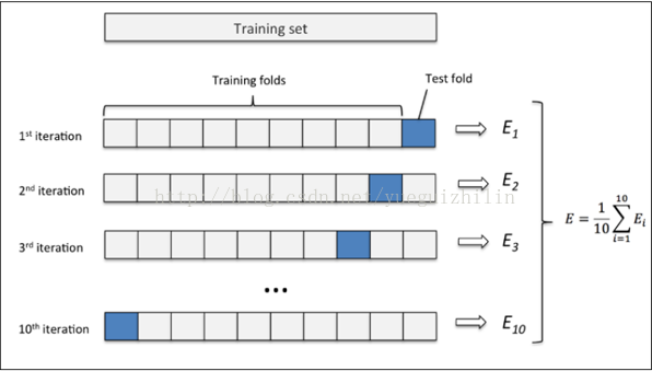
所谓k折交叉验证,就是将训练集随机分为K份,然后,我们依次选择其中的k-1份来进行训练,剩下的1份用来进行测试,循环k次(每次组合的K-1份都不相同),然后取最后的平均精度,作为当前训练出的模型的精度。
我们可以通过Sklearn 中的的 sklearn.cross_validation模块下的train_test_split来随机划分训练集和测试集。
调用方式为:X_train,X_test, y_train, y_test =train_test_split(train_data,train_target,test_size=0.4, random_state=0) 参数说明:
train_data:要划分的样本特征集
train_target:划分的样本输出
test_size: 如果是小数的话,表示划分的测试集所占的样本比例,整数的话,则为测试集样本个数
random_state: 随机数种子,其实就是该组随机数的编号,在需要重复试验的时候,保证得到一组一样的随机数。比如你每次都填1,其他参数一样的情况下你得到的随机数组是一样的。但填0或不填,每次都会不一样。
from sklearn.cross_validation import train_test_split

#这个是将下采样之前的初始样本数据进行训练集和测试集的划分,
X_train, X_test, y_train, y_test = train_test_split(X,y,test_size=0.3, random_state=0)

X_train_under_sample, X_test_under_sample, y_train_under_sample, y_test_under_sample = train_test_split(X_under_sample,
                                                                                                        y_under_sample,
                                                                                                        test_size=0.3,
                                                                                                        random_state=0)
print('训练集样本数:',len(X_train_under_sample))
print('测试集样本数:',len(X_test_under_sample))
训练集样本数: 688
测试集样本数: 296


C:\Anaconda3\lib\site-packages\sklearn\cross_validation.py:41: DeprecationWarning: This module was deprecated in version 0.18 in favor of the model_selection module into which all the refactored classes and functions are moved. Also note that the interface of the new CV iterators are different from that of this module. This module will be removed in 0.20.
  "This module will be removed in 0.20.", DeprecationWarning)
下面,我们将通过交叉验证,采用逻辑回归来训练模型
关于交叉验证,我们可以用sklearn.cross_validation模块中的KFold方法来进行处理。调用方式为:
class sklearn.cross_validation.KFold(n, n_folds=3, shuffle=False, random_state=None)
参数说明:
n:要分割的数据集个数
n_folds: 对应交叉验证折数
shuffle:是否在划分之前洗牌数据。
模型训练与选择
from sklearn.linear_model import LogisticRegression
from sklearn.cross_validation import KFold, cross_val_score
from sklearn.metrics import confusion_matrix,recall_score,classification_report

def Kfold_for_TrainModel(X_train_data, y_train_data):
    fold = KFold(len(X_train_data),5,shuffle = False)

    # 正则化前面的C 参数
    c_params = [0.01, 0.1, 1, 10, 100]
    #这块生成一个DataFrame 用来保存不同的C参数,对应的召回率是多少
    result_tables = pd.DataFrame(columns = ['C_parameter','Mean recall score'])
    result_tables['C_parameter'] = c_params
    j = 0
    for c_param in c_params:
        print('-------------------------------------------')
        print('C参数为:',c_param)
        print('-------------------------------------------')
        print('')

        recall_list = []
        for iteration, indices in enumerate(fold,start=1):
            #采用l1正则化
            lr = LogisticRegression(C=c_param, penalty = 'l1')
            #indices[0] 保存的是这个k=5次训练中的某一次的用来验证的数据的索引
            #indices[1] 保存的是这个k=5次训练中的某一次的用来测试的数据的索引
            lr.fit(X_train_data.iloc[indices[0],:],
                   y_train_data.iloc[indices[0],:].values.ravel())#.ravel可以将输出降到一维
            #用剩下的一份数据进行测试(即indices[1]中所保存的下标)
            y_undersample_pred = lr.predict(X_train_data.iloc[indices[1],:].values)

            recall = recall_score(y_train_data.iloc[indices[1],:].values,
                                  y_undersample_pred)
            recall_list.append(recall)
            print('Iteration ',iteration," 召回率为:",recall)
        print('')
        print('平均召回率为:', np.mean(recall_list))
        print('')
        result_tables.loc[j,'Mean recall score'] = np.mean(recall_list)
        j = j+1

#     print(result_tables['Mean recall score'])
    result_tables['Mean recall score'] = result_tables['Mean recall score'].astype('float64')
    best_c_param = result_tables.loc[result_tables['Mean recall score'].idxmax(), 'C_parameter']
    print('*********************************************************************************')
    print('最佳模型对应的C参数 = ', best_c_param)
    print('*********************************************************************************')
    return best_c_param
best_c_param = Kfold_for_TrainModel(X_train_under_sample, y_train_under_sample)
-------------------------------------------
C参数为: 0.01
-------------------------------------------

Iteration  1  召回率为: 0.9315068493150684
Iteration  2  召回率为: 0.9178082191780822
Iteration  3  召回率为: 1.0
Iteration  4  召回率为: 0.972972972972973
Iteration  5  召回率为: 0.9545454545454546

平均召回率为: 0.9553666992023157

-------------------------------------------
C参数为: 0.1
-------------------------------------------

Iteration  1  召回率为: 0.8356164383561644
Iteration  2  召回率为: 0.863013698630137
Iteration  3  召回率为: 0.9491525423728814
Iteration  4  召回率为: 0.9459459459459459
Iteration  5  召回率为: 0.9090909090909091

平均召回率为: 0.9005639068792076

-------------------------------------------
C参数为: 1
-------------------------------------------

Iteration  1  召回率为: 0.8493150684931506
Iteration  2  召回率为: 0.8904109589041096
Iteration  3  召回率为: 0.9830508474576272
Iteration  4  召回率为: 0.9459459459459459
Iteration  5  召回率为: 0.9090909090909091

平均召回率为: 0.9155627459783485

-------------------------------------------
C参数为: 10
-------------------------------------------

Iteration  1  召回率为: 0.863013698630137
Iteration  2  召回率为: 0.863013698630137
Iteration  3  召回率为: 0.9830508474576272
Iteration  4  召回率为: 0.9459459459459459
Iteration  5  召回率为: 0.8939393939393939

平均召回率为: 0.9097927169206482

-------------------------------------------
C参数为: 100
-------------------------------------------

Iteration  1  召回率为: 0.8767123287671232
Iteration  2  召回率为: 0.863013698630137
Iteration  3  召回率为: 0.9661016949152542
Iteration  4  召回率为: 0.9459459459459459
Iteration  5  召回率为: 0.8939393939393939

平均召回率为: 0.9091426124395708

*********************************************************************************
最佳模型对应的C参数 =  0.01
*********************************************************************************
当正则化参数C设置为0.01时,所得模型的召回率最高。所以我们选择f1正则,并且正则参数为0.01这个模型来作为最终模型。然后接下来,我们将会用最终所训练出的模型,对最终的测试集进行预测。看看效果如何
性能度量
首先,需要说下分类问题中的性能度量相关的东西。那就是混淆矩阵,在混淆矩阵中,我们可以获得很多性能度量相关有用的信息。
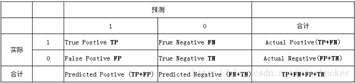
在机器学习中,混淆矩阵(confusion matrix)是一种评价分类模型好坏的形象化展示工具。其中,行代表的是实际类别,列代表的是预测的类别
下面来说下解释下TP,FP,TN和FN
TP(True Positive):真正例,即将一个实际为正例的样本正确的判断为正例
FP(False Positive):假正例,即将一个实际为负例的样本错误的判断为正例
TN(True Negtive):真负例,即将一个实际为负例的样本正确的判断为负例
FN(False Negtive):假负例,即将一个实际为正例的样本错误的判断为负例
下面再介绍几种常用的性能度量的指标
查准率(Precision): 预测为正例的样本中,实际为正例所占的比例,公式为:
查全率(也叫做召回率)(Recall): 正确预测为正例的样本数占所有正例的比率,公式为:
准确率(Accuracy): 所有样本中,预测正确的所占的比例,公式为:
下面,我们来绘制下稀疏矩阵
import itertools
def plot_confusion_matrix(confusion_matrix, classes):
#     print(confusion_matrix)
    #plt.imshow 绘制热图
    plt.figure()
    plt.imshow(confusion_matrix, interpolation='nearest',cmap=plt.cm.Blues)
    plt.title('confusion matrix')
    plt.colorbar()
    tick_marks = np.arange(len(classes))
    plt.xticks(tick_marks, classes, rotation=0)
    plt.yticks(tick_marks, classes)
    thresh = confusion_matrix.max() / 2.
    for i, j in itertools.product(range(confusion_matrix.shape[0]), range(confusion_matrix.shape[1])):
        plt.text(j, i, confusion_matrix[i, j],
                 horizontalalignment="center",
                 color="white" if confusion_matrix[i, j] > thresh else "black")

    plt.tight_layout()
    plt.ylabel('True label')
    plt.xlabel('Predicted label')
    plt.show()
    print('查准率为:',confusion_matrix[1,1]/(confusion_matrix[1,1]+confusion_matrix[0,1]))
    print('召回率为:',confusion_matrix[1,1]/(confusion_matrix[1,1]+confusion_matrix[1,0]))
    print('准确率为:',(confusion_matrix[0,0]+confusion_matrix[1,1])/(confusion_matrix[0,0]+confusion_matrix[0,1]+confusion_matrix[1,1]+confusion_matrix[1,0]))
    print('*********************************************************************************')
lr = LogisticRegression(C = best_c_param, penalty = 'l1')
lr.fit(X_train_under_sample, y_train_under_sample.values.ravel())

#获得测试集的测试结果
y_undersample_pred = lr.predict(X_test_under_sample.values)
#构建稀疏矩阵
conf_matrix = confusion_matrix(y_test_under_sample,y_undersample_pred)
# np.set_printoptions(precision=2)
class_names = [0,1]

plot_confusion_matrix(conf_matrix
                      , classes=class_names)
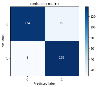
查准率为: 0.9019607843137255
召回率为: 0.9387755102040817
准确率为: 0.918918918918919
*********************************************************************************
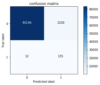
上面求得的度量指标都是针对于下采样样本中的测试集,而我们最后需要测试的是整个所有样本数据中的测试集,所以,下面,我们用刚才训练出来的那个模型,去测试下下采样前的测试集看看
#获得测试集的测试结果
y_pred = lr.predict(X_test.values)
#构建稀疏矩阵
conf_matrix = confusion_matrix(y_test,y_pred)
# np.set_printoptions(precision=2)
class_names = [0,1]

plot_confusion_matrix(conf_matrix
                      , classes=class_names)
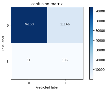
查准率为: 0.012054600248182947
召回率为: 0.9251700680272109
准确率为: 0.8694217197429865
*********************************************************************************
虽然召回率和准确率都不错,但是精确率太低了,也就是说,虽然把147个正样本中的136个都已正确预测出,但是代价是,同时把10894个负例预测为正例。真是宁可错杀一千,也不放过一个啊·
我们想想,为啥会出现这个问题?其实就是因为我们选取的负样本太少了,284315个负样本中,我们只选取了492个来进行训练模型,从而导致泛化能力太差。 这也就是下采样的缺点 由于采样的样本要少于原样本集合,因此会造成一些信息缺失,未被采样的样本往往带有很重要的信息
过采样,SMOTE算法
下面,我们采用过采样,SMOTE算法进行数据的处理
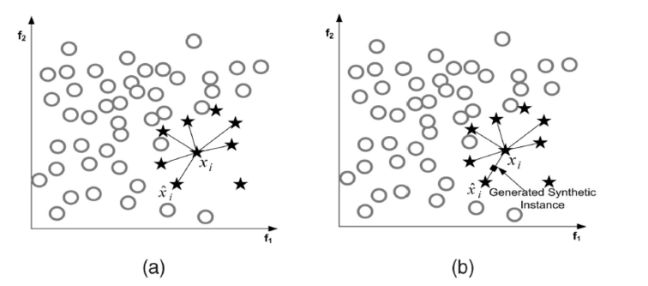
SMOTE全称是Synthetic Minority Oversampling Technique即合成少数类过采样技术,具体思想是:对少数类样本进行分析并根据少数类样本人工合成新样本添加到数据集中
算法流程如下:
- 对于少数类中的每一个样本
,用欧式距离为标准计算它到少数类样本集
中所有样本的距离,得到其k近邻
- 确定采样倍率
,对于每一个少数类样本
SMOTE全称是Synthetic Minority Oversampling Technique即合成少数类过采样技术,具体思想是:对少数类样本进行分析并根据少数类样本人工合成新样本添加到数据集中
算法流程如下:
- 对于少数类中的每一个样本
中所有样本的距离,得到其k近邻
- 确定采样倍率
- 对于每一个随机选出的近邻
,分别与原样本按照如下的公式构建新的样本
下面,看下具体代码
#pip install imblearn 需要先安装imblearn包
from imblearn.over_sampling import SMOTE
from sklearn.ensemble import RandomForestClassifier
oversampler = SMOTE(random_state = 0)

X_over_samples, y_over_samples = oversampler.fit_sample(X_train, y_train.values.ravel())
查下经过过采样,SMOTE算法后,正负样本分别有多少个
len(y_over_samples[y_over_samples == 1]), len(y_over_samples[y_over_samples == 0])
(199019, 199019)
可以看到正负样本已经很均衡了,好了,现在用新的样本集重新进行模型的训练与选择
#这块注意,之前定义的Kfold_for_TrainModel函数传的参数类型是DataFrame,所有这块需要转换下
best_c_param = Kfold_for_TrainModel(pd.DataFrame(X_over_samples),
                                    pd.DataFrame(y_over_samples))
-------------------------------------------
C参数为: 0.01
-------------------------------------------

Iteration  1  召回率为: 0.9285714285714286
Iteration  2  召回率为: 0.912
Iteration  3  召回率为: 0.9129489124936773
Iteration  4  召回率为: 0.8972829022573392
Iteration  5  召回率为: 0.8974462044795055

平均召回率为: 0.9096498895603901

-------------------------------------------
C参数为: 0.1
-------------------------------------------

Iteration  1  召回率为: 0.9285714285714286
Iteration  2  召回率为: 0.92
Iteration  3  召回率为: 0.9145422357106727
Iteration  4  召回率为: 0.8986521285816574
Iteration  5  召回率为: 0.8987777456756315

平均召回率为: 0.9121087077078782

-------------------------------------------
C参数为: 1
-------------------------------------------

Iteration  1  召回率为: 0.9285714285714286
Iteration  2  召回率为: 0.92
Iteration  3  召回率为: 0.9146686899342438
Iteration  4  召回率为: 0.8987777456756315
Iteration  5  召回率为: 0.8989536096071954

平均召回率为: 0.9121942947576999

-------------------------------------------
C参数为: 10
-------------------------------------------

Iteration  1  召回率为: 0.9285714285714286
Iteration  2  召回率为: 0.92
Iteration  3  召回率为: 0.9146686899342438
Iteration  4  召回率为: 0.8988028690944264
Iteration  5  召回率为: 0.8991294735387592

平均召回率为: 0.9122344922277715

-------------------------------------------
C参数为: 100
-------------------------------------------

Iteration  1  召回率为: 0.9285714285714286
Iteration  2  召回率为: 0.92
Iteration  3  召回率为: 0.9146686899342438
Iteration  4  召回率为: 0.8991169118293617
Iteration  5  召回率为: 0.8989661713165927

平均召回率为: 0.9122646403303254

*********************************************************************************
最佳模型对应的C参数 =  100.0
*********************************************************************************
可以看到,当C参数为100时,模型召回率最好,我们就用此模型,进行测试集数据的预测
lr = LogisticRegression(C = best_c_param, penalty = 'l1')
lr.fit(X_over_samples, y_over_samples)
# lr.fit(pd.DataFrame(X_over_samples),  pd.DataFrame(y_over_samples).values.ravel())
#获得测试集的测试结果
y_pred = lr.predict(X_test.values)
#构建稀疏矩阵
conf_matrix = confusion_matrix(y_test,y_pred)
# np.set_printoptions(precision=2)
class_names = [0,1]

plot_confusion_matrix(conf_matrix
                      , classes=class_names)
查准率为: 0.06040268456375839
召回率为: 0.9183673469387755
准确率为: 0.9752817667918964
*********************************************************************************
相对于上面的欠采样,这次效果明显好多了。
欢迎关注我的个人公众号 AI计算机视觉工坊,本公众号不定期推送机器学习,深度学习,计算机视觉等相关文章,欢迎大家和我一起学习,交流。